

Lesson 20: Feature Detection and Matching
This begins Part 2: classical 3D computer vision, where the algorithms increasingly work across multiple images of a scene — video frames, or several cameras — rather than a single one. The first problem that creates: two images of the same scene rarely put the same content at the same pixel location, since rotation, scale, and viewpoint all shift things around. This lesson builds toward feature-based matching, which survives exactly those changes: first corner detectors (Harris, Shi-Tomasi) that find distinctive, repeatable points, then SIFT, which adds scale-invariance and a descriptor that can be matched between two different-looking images of the same scene.
import numpy as np
import cv2
import matplotlib.pyplot as plt
The structure tensor: what makes a good point to match?
At each pixel, build the $2\times2$ structure tensor from the local window of gradients (Lesson 12):
$$M = \sum_{\text{window}} \begin{bmatrix}I_x^2 & I_xI_y \\ I_xI_y & I_y^2\end{bmatrix}$$
This should look familiar: it's exactly the moment covariance matrix from Lesson 6, but built from gradients instead of pixel coordinates. Its eigenvalues $\lambda_1 \ge \lambda_2$ describe the local intensity structure:
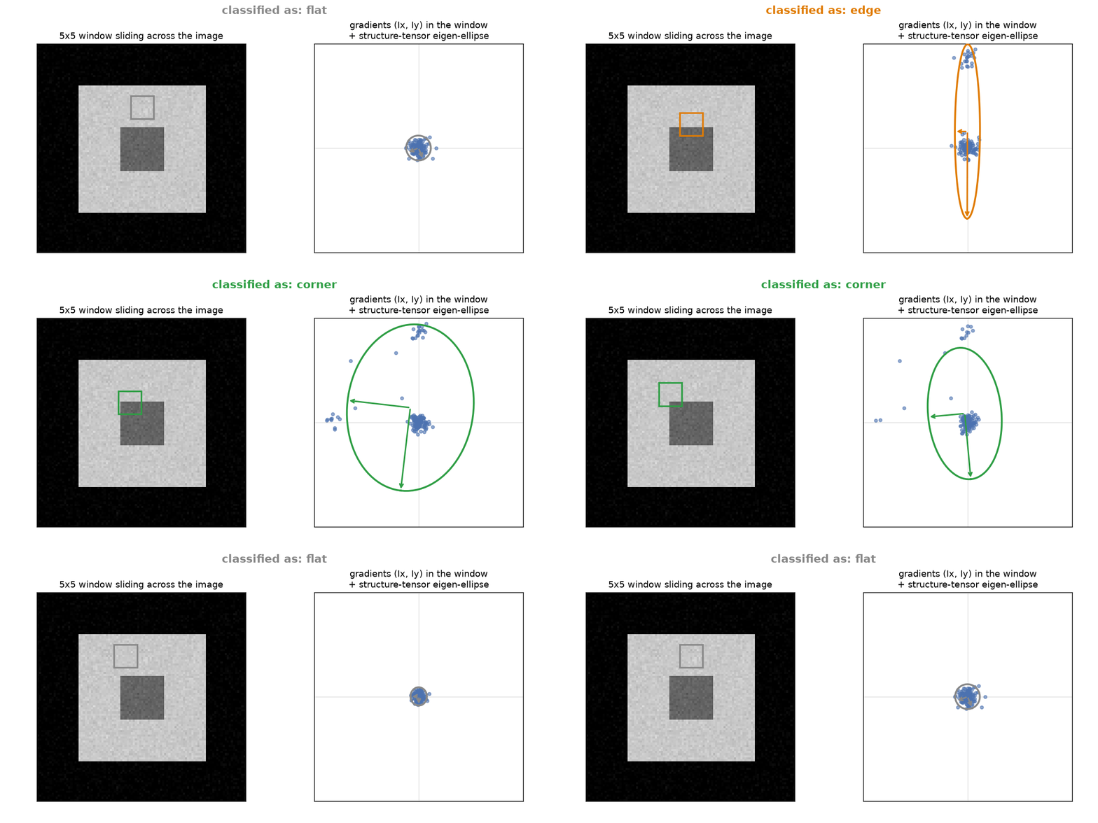
- both small: flat region, gradients weak in every direction
- one large, one small: edge, gradient strong perpendicular to the edge, weak along it
- both large: corner, gradient strong in every direction — exactly the kind of point that can be precisely relocalized in another image
img = np.zeros((100, 100), dtype=np.uint8)
cv2.rectangle(img, (20, 20), (80, 80), 200, -1)
cv2.rectangle(img, (40, 40), (60, 60), 100, -1)
img_f = img.astype(np.float64)

Ix = cv2.Sobel(img_f, cv2.CV_64F, 1, 0, ksize=3)
Iy = cv2.Sobel(img_f, cv2.CV_64F, 0, 1, ksize=3)

window = 5
Sxx = cv2.boxFilter(Ix * Ix, -1, (window, window))
Syy = cv2.boxFilter(Iy * Iy, -1, (window, window))
Sxy = cv2.boxFilter(Ix * Iy, -1, (window, window))

plt.imshow(img, cmap='gray')
plt.title('Test image: corners, edges, and flat regions')
plt.axis('off')
plt.show()

This animation slides the same 5x5 window around this image (with a little pixel noise added so the gradient scatter is an actual cloud of points) — the gradient scatter and its structure-tensor eigen-ellipse update live, and the classification (flat / edge / corner) follows directly from the two eigenvalues, exactly the rule above.
Harris corner detector
Directly computing eigenvalues everywhere is a bit expensive, so Harris and Stephens (1988) proposed a cheaper proxy using only $\det(M)$ and $\text{trace}(M)$ (which can be computed without ever finding eigenvalues):
$$R = \det(M) - k \cdot \text{trace}(M)^2, \qquad k \approx 0.04$$
$R$ is large and positive at corners, negative at edges, and near zero on flat regions.
k = 0.04
det_M = Sxx * Syy - Sxy**2
trace_M = Sxx + Syy
harris_response = det_M - k * trace_M**2

harris_cv = cv2.cornerHarris(img_f.astype(np.float32), blockSize=window, ksize=3, k=k)
print('correlation with cv2.cornerHarris:', np.corrcoef(harris_response.ravel(), harris_cv.ravel())[0, 1])

fig, axes = plt.subplots(1, 2, figsize=(7, 3.5))
axes[0].imshow(img, cmap='gray')
axes[0].set_title('Image')
im = axes[1].imshow(harris_response, cmap='coolwarm')
axes[1].set_title('Harris response R\n(red=corner, blue=edge)')
for ax in axes:
    ax.axis('off')
plt.tight_layout()
plt.show()

Shi-Tomasi: "Good Features to Track"
Shi and Tomasi (1994) argued for using the minimum eigenvalue of $M$ directly instead of Harris's determinant/trace proxy:
$$R_{\text{ST}} = \min(\lambda_1, \lambda_2)$$
A point is only a strong corner if both eigenvalues are large — the minimum being large is exactly that condition, and (unlike Harris's $R$) it has a direct, easily interpretable meaning: it's proportional to the worst-case tracking precision in any direction.
discriminant = np.sqrt(np.clip((trace_M / 2)**2 - det_M, 0, None))
lambda_min = trace_M / 2 - discriminant

eigval_cv = cv2.cornerMinEigenVal(img_f.astype(np.float32), blockSize=window, ksize=3)
print('correlation with cv2.cornerMinEigenVal:', np.corrcoef(lambda_min.ravel(), eigval_cv.ravel())[0, 1])

corners = cv2.goodFeaturesToTrack(img_f.astype(np.uint8), maxCorners=20, qualityLevel=0.1, minDistance=5)

plt.imshow(img, cmap='gray')
for pt in corners[:, 0]:
    plt.scatter(*pt, c='red', s=40, marker='+')
plt.title('cv2.goodFeaturesToTrack (Shi-Tomasi)')
plt.axis('off')
plt.show()

The scale problem
Harris and Shi-Tomasi both operate at a single, fixed window size. Zoom the same corner in or out, and it may stop looking like a corner at that fixed scale (a sharp corner becomes a gentle curve when zoomed out enough) — these detectors are not scale-invariant. SIFT (Scale-Invariant Feature Transform) (Lowe, 1999/2004★) fixes this by searching for keypoints across an entire scale-space, not just one window size.
SIFT: scale-space extrema and descriptors
SIFT's pipeline, at a glance:
- Build a Difference-of-Gaussians (DoG) scale-space — exactly the DoG approximation to the Laplacian from Lesson 13, computed at many blur levels.
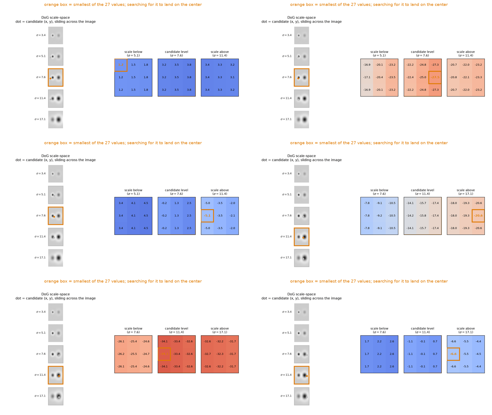
- Find keypoints as local extrema of DoG response across both space and scale — a point that's a maximum compared to its 26 neighbors (including 8 neighbors in the current scale and 9 neighbors in each scale level up and down).
- Assign each keypoint a dominant orientation from the local gradient histogram, so descriptors can be made rotation-invariant.
- Build a 128-dimensional descriptor from histograms of gradient orientations in a $4\times4$ grid of subregions around the keypoint.
The result: a keypoint with a position, a scale, an orientation, and a descriptor vector that's designed to be very similar between two images even under moderate rotation, scaling, and illumination change.
This animation shows the 26-neighbor extremum test on a synthetic Difference-of-Gaussians scale-space with two blobs of different sizes. On the left, the dot marks the candidate pixel's (x, y) location as it slides across the image at different scales. On the right, the three patches show the candidate's 26 neighbors (8 in the same scale plus the matching 3x3 patches one scale level up and down). An orange box highlights the smallest of all 27 values. When the extremum is off-center, the candidate pixel is not a keypoint. The box turns green only when the extremum lands exactly on the candidate pixel: the center of the smaller blob at a smaller sigma, and the center of the larger blob (twice the radius) a full octave later — exactly the scale-selection that fixes the scale problem raised above.
textured = cv2.imread('../img/building.png', cv2.IMREAD_GRAYSCALE)
textured = cv2.cvtColor(textured, cv2.COLOR_BGR2RGB)

sift = cv2.SIFT_create()
keypoints, descriptors = sift.detectAndCompute(textured, None)
print(f'found {len(keypoints)} keypoints, each with a {descriptors.shape[1]}-dim descriptor')

keypoint_vis = cv2.drawKeypoints(textured, keypoints, None,
                                  flags=cv2.DRAW_MATCHES_FLAGS_DRAW_RICH_KEYPOINTS)

fig, axes = plt.subplots(1, 2, figsize=(10, 5))
axes[0].imshow(textured)
axes[0].set_title('Original')
axes[1].imshow(keypoint_vis)
axes[1].set_title('SIFT keypoints (circle size = scale, line = orientation)')
for ax in axes:
    ax.axis('off')
plt.tight_layout()
plt.show()

Photo by Dawson Lovell on Unsplash
Matching under rotation and scale
We rotate and shrink the image with a known transform, detect SIFT features independently in both, then match descriptors with a nearest-neighbor search. Lowe's ratio test keeps a match only if the best candidate is meaningfully closer than the second-best candidate — a simple, effective way to reject ambiguous matches.
M = cv2.getRotationMatrix2D((150, 150), angle=35, scale=0.7)
rotated_scaled = cv2.warpAffine(textured, M, (300, 300))

kp1, des1 = sift.detectAndCompute(textured, None)
kp2, des2 = sift.detectAndCompute(rotated_scaled, None)

bf = cv2.BFMatcher()
raw_matches = bf.knnMatch(des1, des2, k=2)
good_matches = [m for m, n in raw_matches if m.distance < 0.75 * n.distance]

print(f'keypoints: {len(kp1)} (original), {len(kp2)} (rotated + scaled)')
print(f'good matches after Lowe ratio test: {len(good_matches)} / {len(raw_matches)} candidate pairs')
How many matches are actually correct?
Because we know the exact transform M used to create the second image, we can directly check: does mapping each matched keypoint through M land near where it was actually matched?
correct = 0
for m in good_matches:
    p1 = np.array(kp1[m.queryIdx].pt + (1,))
    p2 = np.array(kp2[m.trainIdx].pt)
    predicted = M @ p1
    if np.linalg.norm(predicted - p2) < 3:
        correct += 1

print(f'geometrically correct matches: {correct} / {len(good_matches)} ({100 * correct / len(good_matches):.0f}%)')

match_vis = cv2.drawMatches(textured, kp1, rotated_scaled, kp2, good_matches, None,
                             flags=cv2.DrawMatchesFlags_NOT_DRAW_SINGLE_POINTS)
plt.figure(figsize=(11, 5))
plt.imshow(match_vis)
plt.title(f'{len(good_matches)} matches across a 35-degree rotation + 0.7x scale change')
plt.axis('off')
plt.show()

Nearly all the ratio-test survivors are genuinely correct correspondences, despite the rotation and scale change — something a detector fixed to one scale and orientation simply couldn't recover. This is exactly what makes SIFT-style features the classic approach for tasks like image stitching, object recognition, and visual localization.
Exercises
- Increase the rotation angle to 90 degrees and the scale to 0.3. Does the number of good matches and the geometric-correctness percentage hold up, or degrade? At what point does SIFT start to struggle?
- Try
cv2.ORB_create()(a much faster, free binary-descriptor alternative to SIFT) withcv2.NORM_HAMMINGin theBFMatcherinstead of the default L2 norm. Compare the number of good matches and qualitatively compare speed using%timeitondetectAndCompute. - Lower the ratio-test threshold from
0.75to0.6. How do the number of good matches and the fraction that are geometrically correct both change? What does this tell you about the threshold's role in a precision/recall tradeoff?