Lesson 36: Evaluating a Classifier¶

Every classifier so far has been evaluated with a single number: overall accuracy. That number hides a lot. This lesson builds a 4-class classifier on a deliberately imbalanced subset of CIFAR-10 — real photographs, not synthetic shapes — and shows why accuracy alone can be misleading, using the tools that reveal what's actually going wrong: the confusion matrix, and per-class precision and recall.

In [1]:

import pickle
import tarfile
import urllib.request
from pathlib import Path

import numpy as np
import torch
import torch.nn as nn
import torch.nn.functional as F
import matplotlib.pyplot as plt

A 4-class, imbalanced dataset¶

Four real photo categories from CIFAR-10 (Krizhevsky, 2009): cat, dog, automobile, and truck. The test set has an even 150 images per class, but the training set is deliberately starved of trucks (90 examples, versus 400 each for the other three) — a stand-in for the common real-world situation where some classes are just rarer to collect than others. Cat and dog are included deliberately as a visually similar pair, regardless of how much training data either gets.

In [2]:

CIFAR_URL = 'https://www.cs.toronto.edu/~kriz/cifar-10-python.tar.gz'
CACHE_ROOT = Path.home() / '.cache' / 'cvintro'
CACHE_DIR = CACHE_ROOT / 'cifar-10-batches-py'

def ensure_cifar10():
    if CACHE_DIR.exists():
        return
    CACHE_ROOT.mkdir(parents=True, exist_ok=True)
    archive_path = CACHE_ROOT / 'cifar-10-python.tar.gz'
    if not archive_path.exists():
        print('Downloading CIFAR-10 (~163 MB, one-time, cached under ~/.cache/cvintro)...')
        urllib.request.urlretrieve(CIFAR_URL, archive_path)
    print('Extracting...')
    with tarfile.open(archive_path) as tar:
        tar.extractall(CACHE_ROOT)

def load_cifar_batch(path):
    with open(path, 'rb') as f:
        d = pickle.load(f, encoding='bytes')
    imgs = d[b'data'].reshape(-1, 3, 32, 32).transpose(0, 2, 3, 1).astype(np.float32) / 255.0
    labels = np.array(d[b'labels'], dtype=np.int64)
    return imgs, labels

ensure_cifar10()

CIFAR_LABELS = ['airplane', 'automobile', 'bird', 'cat', 'deer', 'dog', 'frog', 'horse', 'ship', 'truck']
CLASSES = ['cat', 'dog', 'automobile', 'truck']
CLASS_IDS = {name: CIFAR_LABELS.index(name) for name in CLASSES}

train_imgs, train_labels = [], []
for i in range(1, 6):
    imgs, labels = load_cifar_batch(CACHE_DIR / f'data_batch_{i}')
    train_imgs.append(imgs); train_labels.append(labels)
train_imgs, train_labels = np.concatenate(train_imgs), np.concatenate(train_labels)
test_imgs, test_labels = load_cifar_batch(CACHE_DIR / 'test_batch')

rng = np.random.default_rng(7)

def subset_for_classes(imgs, labels, per_class_counts):
    out_imgs, out_labels = [], []
    for i, name in enumerate(CLASSES):
        idx = np.where(labels == CLASS_IDS[name])[0]
        idx = rng.permutation(idx)[:per_class_counts[name]]
        out_imgs.append(imgs[idx])
        out_labels.append(np.full(len(idx), i, dtype=np.int64))
    out_imgs, out_labels = np.concatenate(out_imgs), np.concatenate(out_labels)
    perm = rng.permutation(len(out_imgs))
    return out_imgs[perm], out_labels[perm]

# training set: cat/dog/automobile well represented, truck deliberately starved
X_train, y_train = subset_for_classes(train_imgs, train_labels,
    {'cat': 400, 'dog': 400, 'automobile': 400, 'truck': 90})
# test set: balanced across all four, so the imbalance is purely a training-time artifact
X_test, y_test = subset_for_classes(test_imgs, test_labels,
    {'cat': 150, 'dog': 150, 'automobile': 150, 'truck': 150})

print('training class counts:', dict(zip(CLASSES, (int(c) for c in np.bincount(y_train, minlength=4)))))
print('test class counts:    ', dict(zip(CLASSES, (int(c) for c in np.bincount(y_test, minlength=4)))))

fig, axes = plt.subplots(1, 4, figsize=(8, 2.2))
for ax, name in zip(axes, CLASSES):
    ax.imshow(X_train[y_train == CLASSES.index(name)][0])
    ax.set_title(name, fontsize=9)
    ax.axis('off')
plt.show()

training class counts: {'cat': 400, 'dog': 400, 'automobile': 400, 'truck': 90}
test class counts:     {'cat': 150, 'dog': 150, 'automobile': 150, 'truck': 150}

No description has been provided for this image

In [3]:

class CNN(nn.Module):
    def __init__(self):
        super().__init__()
        self.conv = nn.Sequential(
            nn.Conv2d(3, 16, 5, padding=2), nn.ReLU(),
            nn.MaxPool2d(2),
            nn.Conv2d(16, 32, 5, padding=2), nn.ReLU(),
            nn.MaxPool2d(2),
            nn.Conv2d(32, 64, 3, padding=1), nn.ReLU(),
            nn.AdaptiveMaxPool2d(1),
        )
        self.fc = nn.Linear(64, 4)

    def forward(self, x):
        return self.fc(self.conv(x).flatten(1))

torch.manual_seed(0)
model = CNN()
opt = torch.optim.Adam(model.parameters(), lr=0.0007)
Xt = torch.tensor(X_train).permute(0, 3, 1, 2); yt = torch.tensor(y_train)
for _ in range(150):
    opt.zero_grad()
    loss = F.cross_entropy(model(Xt), yt)
    loss.backward()
    opt.step()

Xte = torch.tensor(X_test).permute(0, 3, 1, 2)
with torch.no_grad():
    preds = model(Xte).argmax(1).numpy()

acc = (preds == y_test).mean()
print(f'overall test accuracy: {acc:.1%}')

overall test accuracy: 50.3%

Just over 50% overall accuracy, on a 4-class task where chance is 25%, sounds like a reasonable result for a small from-scratch CNN on real photos. It hides something important: the model is not equally good at all four classes.

Confusion matrix¶

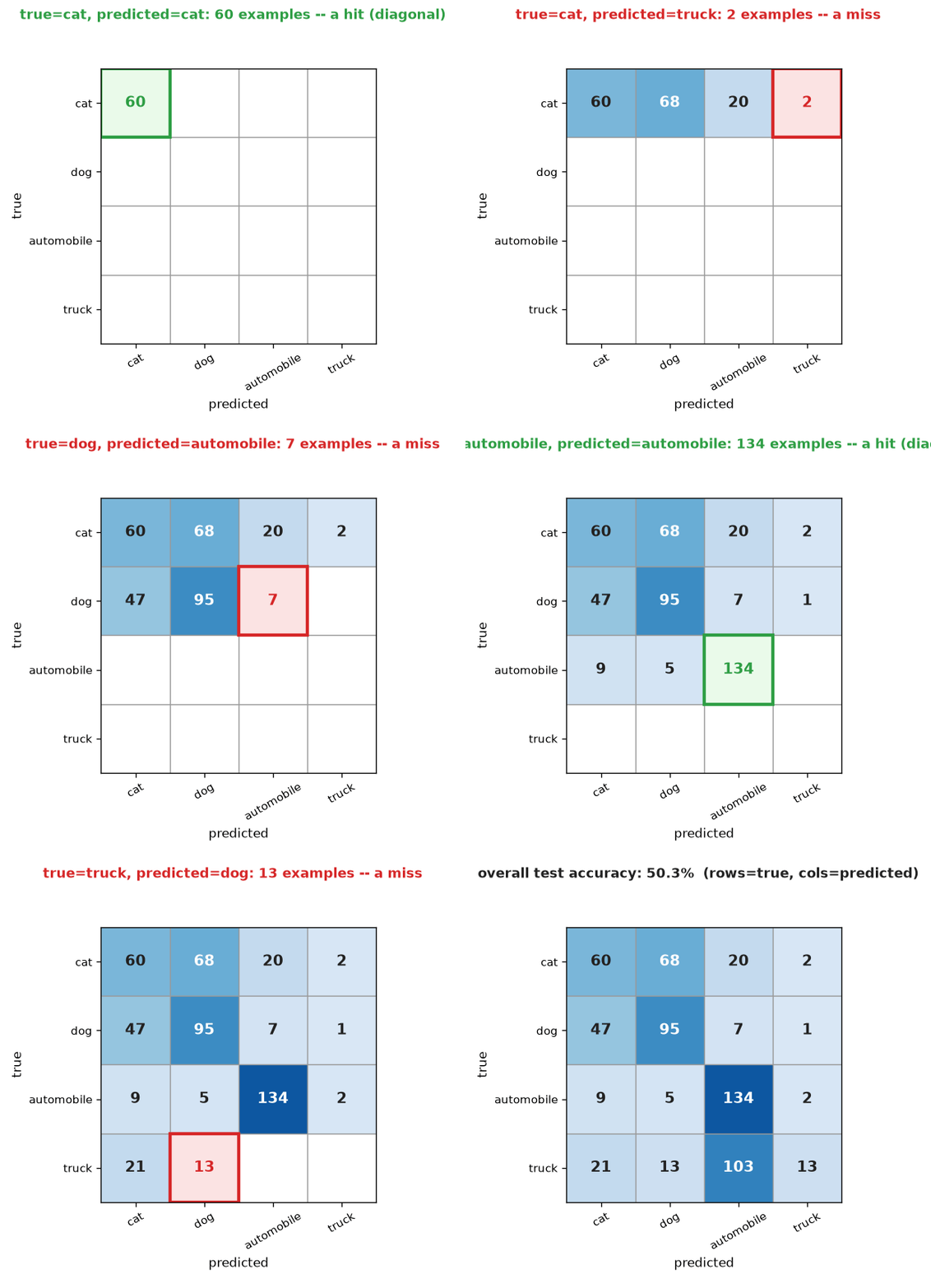
Row i, column j counts test examples of true class i predicted as class j. A perfect classifier is diagonal; everything off the diagonal is a specific, nameable mistake.

In [4]:

cm = np.zeros((4, 4), dtype=int)
for t, p in zip(y_test, preds):
    cm[t, p] += 1

print('confusion matrix (rows=true, cols=predicted):')
print(f'{"":>12}' + ''.join(f'{s:>12}' for s in CLASSES))
for i, s in enumerate(CLASSES):
    print(f'{s:>12}' + ''.join(f'{cm[i, j]:>12}' for j in range(4)))

fig, ax = plt.subplots(figsize=(4.5, 4))
im = ax.imshow(cm, cmap='Blues')
ax.set_xticks(range(4)); ax.set_xticklabels(CLASSES, rotation=45)
ax.set_yticks(range(4)); ax.set_yticklabels(CLASSES)
ax.set_xlabel('predicted'); ax.set_ylabel('true')
for i in range(4):
    for j in range(4):
        ax.text(j, i, cm[i, j], ha='center', va='center',
                 color='white' if cm[i, j] > cm.max() / 2 else 'black')
plt.title('Confusion matrix')
plt.tight_layout()
plt.show()

confusion matrix (rows=true, cols=predicted):
                     cat         dog  automobile       truck
         cat          60          68          20           2
         dog          47          95           7           1
  automobile           9           5         134           2
       truck          21          13         103          13

The animation below fills in the same matrix one cell at a time: green for a hit (on diagonal), red for a miss (off diagonal).

Animated confusion matrix filling in one cell at a time, row by row, with diagonal hits highlighted green and off-diagonal misses highlighted red, ending on the full heatmap

True positives, false positives, true negatives, false negatives¶

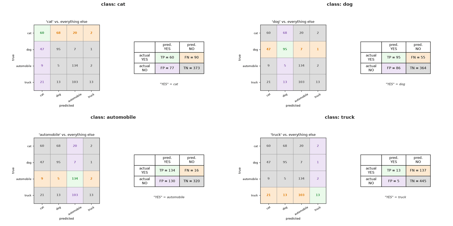
Every cell of the confusion matrix above is a specific kind of correctness or mistake, but the standard vocabulary for talking about them is binary: pick one class and ask only "is it this, or not?" Collapsing the 4-class matrix down to "truck vs. everything else" gives exactly four outcomes:

True positive (TP): actually a truck, predicted truck. A hit.
False negative (FN): actually a truck, predicted something else. A miss — the model let it slip past.
False positive (FP): actually not a truck, predicted truck anyway. A false alarm.
True negative (TN): actually not a truck, correctly predicted not-truck.

This is the same 2x2 table underlying every binary classifier's evaluation (a medical test's "positive/negative" result, a spam filter's "spam/not spam" decision) — a multi-class confusion matrix is just this table computed once per class, with everything off that class's row/column collapsed into "not this class."

In [5]:

cls = CLASSES.index('truck')
tp = cm[cls, cls]
fn = cm[cls, :].sum() - tp          # true truck, predicted something else
fp = cm[:, cls].sum() - tp          # predicted truck, actually something else
tn = cm.sum() - tp - fn - fp        # everything else, correctly not called truck

print(f'{"":>18}{"predicted truck":>20}{"predicted NOT truck":>24}')
print(f'{"actually truck":>18}{tp:>20}{fn:>24}')
print(f'{"actually NOT truck":>18}{fp:>20}{tn:>24}')
print()
print(f'TP={tp}, FP={fp}, FN={fn}, TN={tn}, total={tp+fp+fn+tn} (test set size={len(y_test)})')

                       predicted truck     predicted NOT truck
    actually truck                  13                     137
actually NOT truck                   5                     445

TP=13, FP=5, FN=137, TN=445, total=600 (test set size=600)

The animation below cycles through all four classes, collapsing the full matrix down to each one's TP/FP/FN/TN table — the same collapse performed above for 'truck', generalized.

Animated cycling through each of the four classes, collapsing the full confusion matrix down to that class's TP, FP, FN, TN 2x2 table

Precision and recall¶

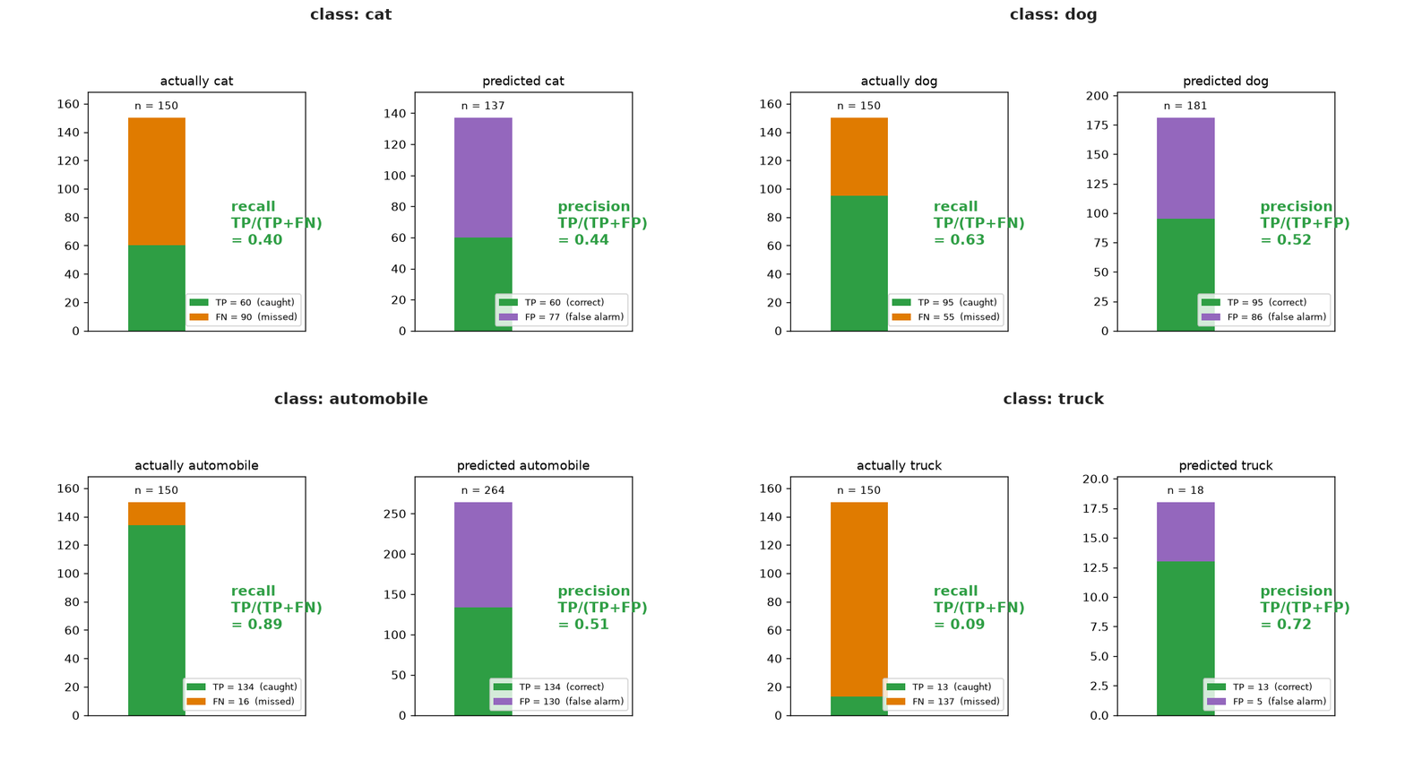
Two numbers per class, computed directly from TP/FP/FN:

Recall = TP / (TP + FN) — of everything that really was class i, what fraction did the model catch? Low recall means the model misses that class often.
Precision = TP / (TP + FP) — of everything the model called class i, what fraction actually was? Low precision means the model cries wolf on that class often.

(A less commonly needed but related pair, built from the other two quadrants: specificity = TN / (TN + FP), how well the model avoids false alarms on the negative class, and its complement the false positive rate = FP / (FP + TN) = 1 − specificity.)

In [6]:

print(f'{"class":>10} {"precision":>10} {"recall":>8} {"support":>8}')
for i, name in enumerate(CLASSES):
    tp = cm[i, i]
    fn = cm[i, :].sum() - tp
    fp = cm[:, i].sum() - tp
    precision = tp / (tp + fp) if (tp + fp) > 0 else float('nan')
    recall = tp / (tp + fn) if (tp + fn) > 0 else float('nan')
    support = cm[i, :].sum()
    print(f'{name:>10} {precision:>10.2f} {recall:>8.2f} {support:>8}')

     class  precision   recall  support
       cat       0.44     0.40      150
       dog       0.52     0.63      150
automobile       0.51     0.89      150
     truck       0.72     0.09      150

The animation below cycles through each class, showing precision and recall as fractions of the same TP/FP/FN counts: a recall bar split into caught (TP) vs. missed (FN), a precision bar split into correct (TP) vs. false alarm (FP).

$Animated cycling through each of the four classes, showing recall as a bar split into true positives and false negatives, and precision as a bar split into true positives and false positives, with the resulting fraction labeled for each$

For quick reference, since these terms go by several names across various fields:

term	formula	also known as
Precision	TP / (TP + FP)	Positive Predictive Value (PPV)
Recall	TP / (TP + FN)	Sensitivity, True Positive Rate (TPR)
Specificity	TN / (TN + FP)	True Negative Rate (TNR)
False Positive Rate	FP / (TN + FP) = 1 − Specificity	Fallout, False Alarm Rate
False Negative Rate	FN / (TP + FN) = 1 − Recall	Miss Rate

Bayes' rule¶

To see why precision behaves the way it does, it may help to recognize a deeper connection. Bayes' rule relates a conditional probability to its reverse: $P(A\mid B) = P(B\mid A)\,P(A)\,/\,P(B)$. Bayes' rule connects precision, $P(\text{actually } i\mid\text{predicted } i)$, with sensitivity/specificity, $P(\text{predicted } i\mid\text{actually } i)$:

$$P(\text{actually } i\mid\text{predicted } i) = \frac{P(\text{predicted } i\mid\text{actually } i)\,P(\text{actually } i)}{P(\text{predicted } i)}.$$

The $P(\text{actually } i)$ term — the base rate or prior, how common class i is to begin with — matters just as much as how good the classifier is.

The classic illustration: a disease with 1% true prevalence, and a test that's "99% accurate" (99% sensitivity, 99% specificity). You test positive — what's the chance you actually have it? Intuition says ≈99%, but the real answer is closer to 50%. The reason: Out of 10,000 people, 100 actually have the disease, and the test catches 99 of them (TP=99). Of the 9,900 healthy people, a 1% false-positive rate flags about 99 more (FP=99) — so among everyone who tests positive, only about half actually has the disease: precision = 99/198 ≈ 50%, nowhere near 99%. A low base rate lets false positives from the enormous healthy majority swamp the true positives from the rare, small minority.

Truck shows the same effect: it's the rarest class here, and even its respectable 72% precision (table above) is already fighting the same uphill arithmetic that makes precision (also known as "positive predictive value") punishing for any rare condition, medical or otherwise.

Precision-recall curve¶

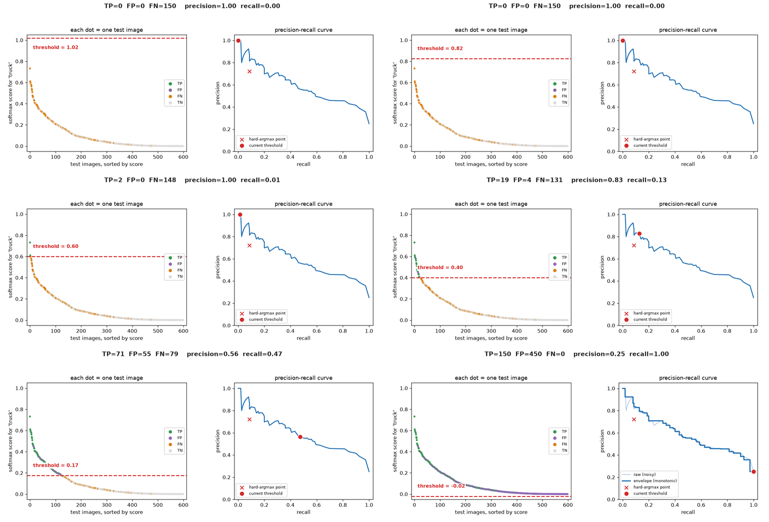
So far, each class's precision and recall came from a single, fixed decision rule: whichever class scores highest wins (hard argmax). But the model doesn't actually output a single verdict — for "truck vs. everything else," it outputs a continuous score (the softmax probability assigned to truck) for every test image. Thresholding that score directly and sweeping the threshold from 0 to 1 traces out a precision-recall curve: the complete tradeoff between catching more trucks and crying wolf less often. Hard argmax isn't quite the same decision rule — it depends on how truck's score compares to the other three classes, not just whether it clears some fixed number — so the point it actually lands on (marked in red) sits close to, but not exactly on, this single-score curve.

The raw curve below is jagged: with so few truck examples, a single unlucky (or lucky) false positive can make precision dip and then recover as the threshold relaxes further, which isn't a real change in the underlying tradeoff — just noise from a small test set. The standard fix (used, for instance, to compute "average precision") is to replace each point's precision with the best precision achieved at that recall or higher, producing a monotonically non-increasing envelope that casts a "shadow" leftward over the noisy dips.

In [7]:

with torch.no_grad():
    probs = F.softmax(model(Xte), dim=1).numpy()

scores = probs[:, cls]          # softmax probability assigned to 'truck'
is_truck = (y_test == cls)

thresholds = np.linspace(0, 1, 101)
precisions, recalls = [], []
for t in thresholds:
    pred_pos = scores >= t
    tp_t = (pred_pos & is_truck).sum()
    fp_t = (pred_pos & ~is_truck).sum()
    fn_t = (~pred_pos & is_truck).sum()
    precisions.append(tp_t / (tp_t + fp_t) if tp_t + fp_t > 0 else 1.0)
    recalls.append(tp_t / (tp_t + fn_t) if tp_t + fn_t > 0 else 0.0)

# the raw curve is jagged (precision isn't monotonic as the threshold relaxes --
# one unlucky false positive can make it dip, then recover). The standard fix,
# used e.g. to compute "average precision": replace each point's precision with
# the BEST precision achieved at that recall or higher -- a monotonically
# non-increasing envelope that "casts a shadow" leftward over the noisy dips.
# Different thresholds can land on the exact same recall (relaxing the
# threshold past a non-truck image changes precision but not recall), so ties
# are first collapsed to their best precision before taking the running max --
# otherwise a later, worse-precision point at the same recall can silently
# undercut an earlier, better one.
order = np.argsort(recalls)
r_sorted = np.array(recalls)[order]
p_sorted = np.array(precisions)[order]
uniq_r, inverse = np.unique(r_sorted, return_inverse=True)
uniq_p = np.zeros_like(uniq_r)
np.maximum.at(uniq_p, inverse, p_sorted)
envelope = np.maximum.accumulate(uniq_p[::-1])[::-1]

plt.plot(recalls, precisions, marker='.', color='#aac4e0', linewidth=1.2, label='raw (noisy)')
# where='pre': each point's value extends LEFTWARD (toward lower recall) onto
# the gap before it -- matching max_{r'>=r} P(r'), and leaving points that are
# already their own local max untouched, instead of dragging a peak forward
# onto later points that don't need it.
plt.step(uniq_r, envelope, where='pre', color='#1f6fb4', linewidth=2.2,
          label='envelope (monotonic)')
plt.scatter([tp / (tp + fn)], [tp / (tp + fp)], color='red', marker='x', s=60, zorder=5,
            label='hard-argmax point')
plt.xlabel('recall'); plt.ylabel('precision')
plt.title('truck: precision-recall curve as the decision threshold sweeps')
plt.legend(fontsize=8)
plt.show()

The animation below makes the mechanism behind that curve concrete: a threshold sweeps across every test image's truck score (sorted left to right), coloring each one TP/FP/FN/TN live as it crosses, while the (recall, precision) point crawls along the same curve shown above.

Animated precision-recall threshold sweep: a decision threshold slides across test images sorted by their softmax truck score, coloring each one as a true positive, false positive, false negative, or true negative as it crosses, while a point traces the resulting precision-recall curve on a second panel

Truck — the class starved to 90 training images, versus 400 for each other class — has high precision but low recall: when the model does say "truck," it's usually right, but it fails to recognize the overwhelming majority of actual trucks, defaulting instead to whichever classes it saw plenty of during training (mostly "automobile," the visually closest well-represented class). That is the standard signature of class imbalance, and it is completely invisible in the single overall-accuracy number from before. Cat and dog, by contrast, are both well-represented in training but get confused with each other far more than with automobile or truck — a different failure mode entirely, caused by genuine visual similarity between the two animals rather than by lack of data. Automobile ends up with unusually high recall but not-so-great precision, for the same reason truck's recall suffered: it's absorbing the starved truck class's misclassifications, since "wheeled vehicle" is an easy fallback guess once the model can't tell trucks apart from automobiles.

The practical lesson: always inspect the confusion matrix and per-class metrics before trusting a single accuracy figure, especially on a dataset where classes aren't balanced.

Exercises¶

Increase the truck training count from 90 to 400 (matching the other three classes) and rerun. Does truck recall recover? Does the cat/dog confusion also improve, or does it persist — and why would more data not fix a problem caused by genuine visual similarity rather than data scarcity?
Try weighting the loss by inverse class frequency (F.cross_entropy(logits, yt, weight=class_weights), where class_weights[i] = 1 / count(class i)) instead of collecting more truck images. Does it recover truck recall, and at what cost to the other classes' precision?
Compute the F1 score (the harmonic mean of precision and recall, 2 * p * r / (p + r)) for each class. Why might F1 be a better single number to track per-class than accuracy, when accuracy is only meaningful in aggregate?

Take the Lesson 36 Quiz →

← Lesson 35: Training a CNN

Lesson 37: Classic Architectures →