

Lesson 20: Optical Flow and Motion Estimation
Optical flow estimates apparent motion between two frames of a video: for each pixel (or a chosen set of points), a 2D vector $(u, v)$ describing where it moved to. This lesson derives the classic Lucas-Kanade method from the same structure tensor used for corner detection in Lesson 19, confronts the fundamental aperture problem, contrasts it with the globally-optimized Horn-Schunck method, and finishes with dense flow via the Farnebäck method.
import numpy as np
import cv2
import matplotlib.pyplot as plt
The brightness constancy assumption
Optical flow assumes a point's intensity doesn't change as it moves: $I(x, y, t) = I(x+u, y+v, t+1)$. A first-order Taylor expansion of the right side gives the optical flow constraint equation:
$$I_x u + I_y v + I_t = 0$$
where $I_x, I_y$ are the spatial gradients (Lesson 12) and $I_t$ is the frame-to-frame intensity difference. This is one equation with two unknowns (the motion $u$ and $v$) at every single pixel — not enough information on its own to solve for the flow.
The aperture problem
Looking through a small window at a moving edge, only the motion perpendicular to the edge is visible; motion along the edge produces no visible change at all, and so is invisible to a local measurement. This is exactly why the flow constraint equation is underdetermined: it only ever constrains the component of $(u,v)$ along the gradient direction $(I_x, I_y)$, leaving the perpendicular component completely unconstrained by that one equation.
size = 160
rect_topleft = (50, 60)
rect_w, rect_h = 60, 40

def make_rect_frame(dx=0, dy=0, value=200):
    img = np.zeros((size, size), dtype=np.uint8)
    x0, y0 = rect_topleft[0] + dx, rect_topleft[1] + dy
    cv2.rectangle(img, (x0, y0), (x0 + rect_w, y0 + rect_h), value, -1)
    return img

true_motion = (8, 6)           # right and down
vertical_only_motion = (0, 6)  # same downward shift, but no horizontal component

frame_true = make_rect_frame(*true_motion)
frame_vertical = make_rect_frame(*vertical_only_motion)

# A small aperture window straddling the rectangle's TOP (horizontal) edge, centered well
# away from any corner and comfortably inside the canvas, so there are no border effects.
win_half = 10
wx, wy = rect_topleft[0] + rect_w // 2, rect_topleft[1]

def with_window(img_gray, color=(255, 0, 0)):
    vis = cv2.cvtColor(img_gray, cv2.COLOR_GRAY2RGB)
    cv2.rectangle(vis, (wx - win_half, wy - win_half), (wx + win_half, wy + win_half), color, 1)
    return vis

fig, axes = plt.subplots(1, 2, figsize=(7, 4))
axes[0].imshow(with_window(frame_true))
axes[0].set_title(f'True motion (u,v)={true_motion}\n(right + down)', fontsize=9)
axes[1].imshow(with_window(frame_vertical))
axes[1].set_title(f'Vertical-only motion (u,v)={vertical_only_motion}\n(down only)', fontsize=9)
for ax in axes:
    ax.axis('off')
plt.tight_layout()
plt.show()

window_true = frame_true[wy - win_half:wy + win_half, wx - win_half:wx + win_half]
window_vertical = frame_vertical[wy - win_half:wy + win_half, wx - win_half:wx + win_half]
print('inside the red window, the two (different!) motions look pixel-for-pixel identical:',
      np.array_equal(window_true, window_vertical))

Both frames actually show a different global motion — one moves right and down, the other only down — yet inside the red window (which straddles the rectangle's top edge, a purely horizontal edge) they're indistinguishable. The horizontal component is along that edge, so it leaves no trace locally; only the shared vertical component, perpendicular to the edge, is visible. A local measurement at this window genuinely cannot tell these two motions apart.
Lucas-Kanade: solving the aperture problem with a window
Lucas and Kanade's fix (1981): assume the flow $(u,v)$ is constant over a small window, then combine the flow constraint equation from every pixel in that window into an overdetermined least-squares system:
$$\underbrace{\begin{bmatrix}\sum I_x^2 & \sum I_xI_y \\ \sum I_xI_y & \sum I_y^2\end{bmatrix}}_{M}\begin{bmatrix}u\\v\end{bmatrix} = -\begin{bmatrix}\sum I_xI_t\\ \sum I_yI_t\end{bmatrix}$$
$M$ is exactly the structure tensor from Lesson 19! This is not a coincidence: solving this system requires $M$ to be invertible, i.e. to have two large eigenvalues — precisely the Shi-Tomasi "good feature to track" condition. A flat region ($M$ near zero) or an edge (one small eigenvalue — the aperture problem again) gives an ill-conditioned or singular system; a corner gives a well-conditioned one. Corners are trackable for exactly the same reason they're good corners.
rng = np.random.default_rng(0)
frame1 = np.zeros((200, 200), dtype=np.uint8)
for _ in range(20):
    x, y = rng.integers(20, 180, 2)
    radius = rng.integers(5, 15)
    cv2.circle(frame1, (x, y), radius, int(rng.integers(100, 255)), -1)

small_motion = (0.6, 0.4)  # sub-pixel motion, well inside the linear (Taylor) approximation's validity
shift = np.float32([[1, 0, small_motion[0]], [0, 1, small_motion[1]]])
frame2_small = cv2.warpAffine(frame1, shift, (200, 200))

Ix = cv2.Sobel(frame1.astype(np.float64), cv2.CV_64F, 1, 0, ksize=3, scale=1 / 8)
Iy = cv2.Sobel(frame1.astype(np.float64), cv2.CV_64F, 0, 1, ksize=3, scale=1 / 8)
It = frame2_small.astype(np.float64) - frame1.astype(np.float64)


def lucas_kanade_at(x, y, half_win=7):
    x, y = int(round(x)), int(round(y))
    ix = Ix[y - half_win:y + half_win + 1, x - half_win:x + half_win + 1].ravel()
    iy = Iy[y - half_win:y + half_win + 1, x - half_win:x + half_win + 1].ravel()
    it = It[y - half_win:y + half_win + 1, x - half_win:x + half_win + 1].ravel()
    A = np.stack([ix, iy], axis=1)
    solution, *_ = np.linalg.lstsq(A, -it, rcond=None)
    return solution

corners = cv2.goodFeaturesToTrack(frame1, maxCorners=30, qualityLevel=0.1, minDistance=10)
flows = np.array([lucas_kanade_at(p[0][0], p[0][1]) for p in corners])

print(f'true motion:        {small_motion}')
print(f'manual LK estimate: ({flows[:, 0].mean():.3f}, {flows[:, 1].mean():.3f})  (averaged over {len(corners)} corners)')
Visualizing the image, the tracked features, and their motion
arrow_scale = 15  # true motion here is sub-pixel, so exaggerate the arrows to make them visible

vis_small = cv2.cvtColor(frame1, cv2.COLOR_GRAY2RGB)
for (x, y), (u, v) in zip(corners[:, 0], flows):
    p0 = (int(round(x)), int(round(y)))
    p1 = (int(round(x + u * arrow_scale)), int(round(y + v * arrow_scale)))
    cv2.arrowedLine(vis_small, p0, p1, (255, 0, 0), 1, tipLength=0.3)
    cv2.circle(vis_small, p0, 2, (0, 255, 0), -1)

plt.imshow(vis_small)
plt.title(f'Corners (green) and estimated motion (red, {arrow_scale}x exaggerated)\ntrue motion = {small_motion}')
plt.axis('off')
plt.show()

Larger motions need iteration
This single-shot linear solve relies on the Taylor approximation, which only holds for small motions. For a bigger shift, the same one-shot approach degrades:
large_motion = (4.0, 3.0)
shift_large = np.float32([[1, 0, large_motion[0]], [0, 1, large_motion[1]]])
frame2_large = cv2.warpAffine(frame1, shift_large, (200, 200))

It_large = frame2_large.astype(np.float64) - frame1.astype(np.float64)

def lucas_kanade_large(x, y, half_win=7):
    x, y = int(round(x)), int(round(y))
    ix = Ix[y - half_win:y + half_win + 1, x - half_win:x + half_win + 1].ravel()
    iy = Iy[y - half_win:y + half_win + 1, x - half_win:x + half_win + 1].ravel()
    it = It_large[y - half_win:y + half_win + 1, x - half_win:x + half_win + 1].ravel()
    A = np.stack([ix, iy], axis=1)
    solution, *_ = np.linalg.lstsq(A, -it, rcond=None)
    return solution

flows_large_manual = np.array([lucas_kanade_large(p[0][0], p[0][1]) for p in corners])

next_pts, status, _ = cv2.calcOpticalFlowPyrLK(frame1, frame2_large, corners, None, winSize=(15, 15), maxLevel=2)
cv_flow = (next_pts - corners).reshape(-1, 2)[status.ravel() == 1]

print(f'true motion:                          {large_motion}')
print(f'single-shot manual LK estimate:       ({flows_large_manual[:, 0].mean():.3f}, {flows_large_manual[:, 1].mean():.3f})  <- degraded')
print(f'cv2.calcOpticalFlowPyrLK estimate:    ({cv_flow[:, 0].mean():.3f}, {cv_flow[:, 1].mean():.3f})  <- accurate')
OpenCV's calcOpticalFlowPyrLK handles large motions by running Lucas-Kanade iteratively (re-warping and re-linearizing until convergence) on an image pyramid (Lesson 11) — estimate coarsely on a small, blurry version of the image first, then refine level by level. This combination lets it recover large motions accurately even though the underlying linear approximation is only valid locally, one small step at a time.
Visualizing sparse flow vectors
arrow_scale = 3  # exaggerate the arrows a bit so they're easier to see

vis = cv2.cvtColor(frame1, cv2.COLOR_GRAY2RGB)
for (p0,), (p1,), ok in zip(corners, next_pts, status.ravel()):
    if not ok:
        continue
    p0 = p0.astype(int)
    p1_exaggerated = np.round(p0 + (p1 - p0) * arrow_scale).astype(int)
    cv2.arrowedLine(vis, tuple(p0), tuple(p1_exaggerated), (255, 0, 0), 1, tipLength=0.3)
    cv2.circle(vis, tuple(p0), 2, (0, 255, 0), -1)

plt.imshow(vis)
plt.title(f'Tracked corners, true motion = {large_motion} (arrows {arrow_scale}x exaggerated)')
plt.axis('off')
plt.show()

Horn-Schunck: a global alternative to windowed flow
Lucas-Kanade's window is a local smoothness assumption: flow is constant over a small neighborhood, estimated independently at each point. The same year, Horn and Schunck (1981) proposed a global alternative: instead of many independent per-window solves, minimize a single energy over the whole image at once, trading off how well the flow satisfies the optical flow constraint equation against how smoothly it varies between neighboring pixels:
$$E(u,v) = \sum_{x,y} \underbrace{(I_x u + I_y v + I_t)^2}_{\text{data term}} \;+\; \alpha^2 \underbrace{\left(\|\nabla u\|^2 + \|\nabla v\|^2\right)}_{\text{smoothness term}}$$
The smoothness term is what makes this global: it couples every pixel's flow to its neighbors', so minimizing $E$ (e.g., by iterative Gauss-Seidel updates) lets reliable flow estimates near edges propagate into flat, textureless regions that have no local information of their own — exactly the failure mode the aperture problem produces at its worst.
hs_img1 = np.zeros((120, 120), dtype=np.uint8)
cv2.rectangle(hs_img1, (40, 40), (80, 80), 200, -1)  # one textured square, otherwise flat
hs_true_motion = (3.0, 2.0)
hs_shift = np.float32([[1, 0, hs_true_motion[0]], [0, 1, hs_true_motion[1]]])
hs_img2 = cv2.warpAffine(hs_img1, hs_shift, (120, 120))

def horn_schunck(I1, I2, alpha=5.0, n_iters=100):
    Ix = cv2.Sobel(I1.astype(np.float64), cv2.CV_64F, 1, 0, ksize=3, scale=1 / 8)
    Iy = cv2.Sobel(I1.astype(np.float64), cv2.CV_64F, 0, 1, ksize=3, scale=1 / 8)
    It = I2.astype(np.float64) - I1.astype(np.float64)
    u, v = np.zeros_like(Ix), np.zeros_like(Ix)
    neighbor_avg = np.array([[0, 1, 0], [1, 0, 1], [0, 1, 0]], dtype=np.float64) / 4.0
    for _ in range(n_iters):
        u_avg, v_avg = cv2.filter2D(u, -1, neighbor_avg), cv2.filter2D(v, -1, neighbor_avg)
        correction = (Ix * u_avg + Iy * v_avg + It) / (alpha ** 2 + Ix ** 2 + Iy ** 2)
        u, v = u_avg - Ix * correction, v_avg - Iy * correction
    return u, v

fig, axes = plt.subplots(1, 3, figsize=(10, 3.5))
for ax, n_iters in zip(axes, [1, 20, 200]):
    u, v = horn_schunck(hs_img1, hs_img2, n_iters=n_iters)
    magnitude = np.hypot(u, v)
    im = ax.imshow(magnitude, cmap='viridis', vmin=0, vmax=np.hypot(*hs_true_motion))
    ax.set_title(f'{n_iters} iterations', fontsize=9)
    ax.axis('off')
plt.suptitle(f'Flow magnitude spreading outward from the square (true motion = {hs_true_motion})')
plt.tight_layout()
plt.show()

After just 1 iteration, flow is only nonzero right at the square's edges, where there's local gradient information; by 200 iterations that glow has spread well beyond the edges into the surrounding flat region, though it's still far from having reached every pixel — a real solver would run many more iterations (or use a pyramid, the same trick Lucas-Kanade uses for large motions) to converge everywhere. Even this partial spread already shows the mechanism at work: smoothness propagating information into regions with no data term of their own.
Farnebäck's method for dense optical flow
Horn-Schunck's global optimization is elegant but expensive and slow to converge; for dense (every-pixel) flow, Farnebäck's method (2003) — exposed as cv2.calcOpticalFlowFarneback — is a more popular method actually used in practice. It stays local, like Lucas-Kanade, but drops the constant-flow-in-a-window assumption in favor of locally approximating each neighborhood with a polynomial and comparing the polynomial expansions between frames.
dense_motion = (5.0, -3.0)
shift_dense = np.float32([[1, 0, dense_motion[0]], [0, 1, dense_motion[1]]])
frame2_dense = cv2.warpAffine(frame1, shift_dense, (200, 200))

flow = cv2.calcOpticalFlowFarneback(frame1, frame2_dense, None, pyr_scale=0.5, levels=3,
                                     winsize=15, iterations=3, poly_n=5, poly_sigma=1.2, flags=0)

print(f'true motion: {dense_motion}')
print(f'mean flow, ALL pixels:      ({flow[..., 0].mean():.2f}, {flow[..., 1].mean():.2f})  <- biased low')

gradient_mag = np.hypot(cv2.Sobel(frame1.astype(np.float64), cv2.CV_64F, 1, 0, ksize=3),
                         cv2.Sobel(frame1.astype(np.float64), cv2.CV_64F, 0, 1, ksize=3))
textured = gradient_mag > 50
textured[:15, :] = textured[-15:, :] = textured[:, :15] = textured[:, -15:] = False  # avoid warp border artifacts

print(f'mean flow, TEXTURED pixels: ({flow[textured, 0].mean():.2f}, {flow[textured, 1].mean():.2f})  <- accurate')
This is the aperture problem again, at its most extreme: over flat, textureless background, there's no local information at all to estimate motion from, so the flow there is unreliable and drags the whole-image average away from the true value. Restricting to textured (high-gradient) pixels recovers the true motion almost exactly.
def flow_to_color(flow):
    magnitude, angle = cv2.cartToPolar(flow[..., 0], flow[..., 1])
    hsv = np.zeros(flow.shape[:2] + (3,), dtype=np.uint8)
    hsv[..., 0] = angle * 180 / np.pi / 2       # hue = direction
    hsv[..., 1] = 255                            # full saturation
    hsv[..., 2] = cv2.normalize(magnitude, None, 0, 255, cv2.NORM_MINMAX)  # value = speed
    return cv2.cvtColor(hsv, cv2.COLOR_HSV2RGB)

fig, axes = plt.subplots(1, 2, figsize=(7, 3.5))
axes[0].imshow(frame1, cmap='gray')
axes[0].set_title('Frame 1')
axes[1].imshow(flow_to_color(flow))
axes[1].set_title(f'Dense flow field\n(color = direction, brightness = speed)')
for ax in axes:
    ax.axis('off')
plt.tight_layout()
plt.show()

Every moving circle produces the same color, since they all share the same true motion here.
A real video: the Army sequence
On a real video with independently moving objects, this color-coding immediately separates different motions at a glance — exactly why it's the standard way to visualize dense flow fields.
Flickering between the two frames makes the motion easy to see directly — watch how differently the toy soldiers, the ball, and the background shift.
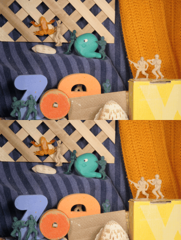
Image source: Middlebury Optical Flow
im1 = cv2.imread('../img/army10.png', cv2.IMREAD_GRAYSCALE)
im2 = cv2.imread('../img/army11.png', cv2.IMREAD_GRAYSCALE)
imflow = cv2.calcOpticalFlowFarneback(im1, im2, None, pyr_scale=0.5, levels=3,
                                     winsize=15, iterations=3, poly_n=5, poly_sigma=1.2, flags=0)

fig, axes = plt.subplots(1, 2, figsize=(7, 3.5))
axes[0].imshow(im1, cmap='gray')
axes[0].set_title('Frame 1')
axes[1].imshow(flow_to_color(imflow))
axes[1].set_title(f'Dense flow field\n(color = direction, brightness = speed)')
for ax in axes:
    ax.axis('off')
plt.tight_layout()
plt.show()

Exercise
- Rerun the sparse Lucas-Kanade comparison with
large_motion = (10.0, 8.0). Doescv2.calcOpticalFlowPyrLKstill recover it accurately? At what point (try increasingly large motions) does it start to fail, and why would you expect a pyramid to help push that limit further out? - Modify the synthetic scene so the circles move with different velocities (e.g. half moving one way, half another). Re-run the dense Farnebäck color visualization and confirm the two motions appear as two distinct colors.
- In the aperture-problem demo, construct a small textured (non-edge) patch instead of a straight edge, and show that both components of an arbitrary motion vector are recoverable from it — unlike the edge case, this should not have an invisible direction of motion.