

Lesson 21: Stereo Matching
Two cameras viewing the same scene from slightly different positions see the same 3D points shifted by different amounts depending on depth — nearby points shift more, distant points shift less. Stereo matching finds these shifts (the disparity) at every pixel, which convert into depth via triangulation. The key problem is correspondence: finding, for every pixel in the left image, the matching pixel in the right. This lesson builds a block matcher that solves it by comparing small patches with sum-of-squared differences (SSD) — a close cousin of Lesson 20's optical flow, but restricted to a 1D search along a single row instead of a full 2D neighborhood.
import numpy as np
import cv2
import matplotlib.pyplot as plt

# shared colormap: invalid/masked-out disparities (NaN) render as gray instead of viridis's default
invalid_cmap = plt.cm.viridis.copy()
invalid_cmap.set_bad('gray')
Rectified stereo: why the search is 1D
For a pair of cameras that are side-by-side, pointed the same direction, with parallel image planes (a rectified stereo pair — real camera rigs are calibrated and warped to approximate this), a fundamental fact of epipolar geometry applies: the corresponding point for any pixel in the left image lies on the same row in the right image. This collapses the search for a match from a 2D image search down to a 1D scan along one row, and the horizontal offset between the two matching positions is the disparity $d$.
Disparity relates to depth by
$$Z = \frac{f \cdot B}{d}$$
where $f$ is the focal length and $B$ is the baseline (distance between the two camera centers). For a rectified pair, depth is inversely proportional to disparity: nearby objects have large disparity, distant objects have small disparity, and an object infinitely far away has zero disparity.
A synthetic stereo pair with known ground truth
We build a left image of pure random texture (so every patch is locally distinctive — no aperture-problem ambiguity) and construct the right image by shifting each pixel left by its true disparity, which we set to three different constant values for three depth "planes": a background and two nearer rectangles. Nearer surfaces shift more than farther ones, so they uncover background pixels on one side that have no corresponding pixel in the left image at all — an occlusion, which we patch with fresh random noise so every right-image pixel still has some value.
rng = np.random.default_rng(0)
h, w = 150, 200
left = rng.integers(0, 255, (h, w)).astype(np.uint8)

true_disparity = np.full((h, w), 5, dtype=np.int32)     # background         (disparity =  5)
true_disparity[30:120, 50:150] = 15                     # a close rectangle  (disparity = 15)
true_disparity[60:90, 80:120] = 25                      # a closer rectangle (disparity = 25)

right = np.full((h, w), -1, dtype=np.int32)
for y in range(h):
    for x in range(w):
        xr = x - true_disparity[y, x]
        if 0 <= xr < w:
            right[y, xr] = left[y, x]
occluded = right == -1   # positions no left pixel maps to: disocclusions, filled with fresh noise
right[occluded] = rng.integers(0, 255, occluded.sum())
right = right.astype(np.uint8)

fig, axes = plt.subplots(1, 3, figsize=(10, 3.5))
axes[0].imshow(left, cmap='gray')
axes[0].set_title('Left image', fontsize=9)
axes[1].imshow(right, cmap='gray')
axes[1].set_title('Right image', fontsize=9)
im = axes[2].imshow(true_disparity, cmap='viridis')
axes[2].set_title('Ground-truth disparity', fontsize=9)
for ax in axes:
    ax.axis('off')
plt.colorbar(im, ax=axes, orientation='vertical', fraction=0.046, pad=0.04, label='disparity (px)')
plt.show()

Block matching along the scanline
For each pixel in the left image, we slide a small window along the same row of the right image over a range of candidate disparities and keep the disparity with the lowest sum-of-squared-differences. The implementation below has three nested Python loops, so it's slow — we run it on a small crop rather than the full image.
def block_match_stereo(left, right, block_size=7, max_disp=30):
    h, w = left.shape
    half = block_size // 2
    left_f, right_f = left.astype(np.float64), right.astype(np.float64)
    disparity_map = np.zeros((h, w), dtype=np.float64)

    for y in range(half, h - half):
        for x in range(half, w - half):
            left_patch = left_f[y - half:y + half + 1, x - half:x + half + 1]
            best_d, best_cost = 0, np.inf
            for d in range(max_disp + 1):
                xr = x - d
                if xr - half < 0:
                    break
                right_patch = right_f[y - half:y + half + 1, xr - half:xr + half + 1]
                cost = ((left_patch - right_patch)**2).sum()
                if cost < best_cost:
                    best_cost, best_d = cost, d
            disparity_map[y, x] = best_d
    return disparity_map

# a small crop, since the pure-Python pixel loop is slow
crop = np.s_[0:100, 0:100]
manual_disp = block_match_stereo(left[crop], right[crop], block_size=7, max_disp=30)

fig, axes = plt.subplots(1, 3, figsize=(10, 3.5))
axes[0].imshow(left[crop], cmap='gray')
axes[0].set_title(f'Left crop ({left[crop].shape[0]}x{left[crop].shape[1]})', fontsize=9)
axes[1].imshow(true_disparity[crop], cmap='viridis', vmin=0, vmax=30)
axes[1].set_title(f'True disparity ({true_disparity[crop].shape[0]}x{true_disparity[crop].shape[1]})', fontsize=9)
im = axes[2].imshow(manual_disp, cmap='viridis', vmin=0, vmax=30)
axes[2].set_title(f'Recovered disparity ({manual_disp.shape[0]}x{manual_disp.shape[1]})', fontsize=9)
for ax in axes:
    ax.axis('off')
plt.colorbar(im, ax=axes, orientation='vertical', fraction=0.046, pad=0.04, label='disparity (px)')
plt.show()

The border along the crop's edges can be ignored: the sliding window runs out of room to search there, an edge effect much like convolution's border handling (Lesson 10). Away from that border, and within the interior of the rectangles, the recovered disparity matches the ground truth almost perfectly, cleanly separating all three depth planes. The exception is the speckled band at each rectangle's edge: a window straddling a depth boundary mixes pixels from two different true disparities, so no single candidate disparity fits the whole window well, and the match becomes unreliable — a preview of the occlusion problem tackled next. Real photos are even less forgiving than this toy case: repetitive texture, flat regions, specular highlights, and shading all add genuine ambiguity on top of occlusion, which is why stereo matching is hard in practice.
Catching bad matches: the left-right consistency check
Occlusions and depth-boundary ambiguity produce wrong matches, like the speckle above. The fix: match both left-to-right and right-to-left, then keep only the pixels where the two results agree, discarding the rest as unreliable. Computing the right-to-left disparity needs no new code — flip both images left-right, swap which one plays "left," run the exact same matcher, then flip the result back. A pixel fails the check whenever the two directions disagree by more than about a pixel. This is especially effective at catching occlusions: a pixel hidden behind a nearer surface in the other view has no true match there at all.
block_size, max_disp = 7, 30
crop_lr = np.s_[0:100, 0:100]
left_c, right_c = left[crop_lr], right[crop_lr]

disp_lr = block_match_stereo(left_c, right_c, block_size=block_size, max_disp=max_disp)
disp_rl = block_match_stereo(right_c[:, ::-1], left_c[:, ::-1], block_size=block_size, max_disp=max_disp)[:, ::-1]

h_c, w_c = disp_lr.shape
consistent = np.zeros((h_c, w_c), dtype=bool)
for y in range(h_c):
    for x in range(w_c):
        d = int(disp_lr[y, x])
        xr = x - d
        if 0 <= xr < w_c:
            consistent[y, x] = abs(disp_rl[y, xr] - d) <= 1

# keep the full crop (no trimming) so the border-truncation effect is visible directly,
# alongside the occlusion-driven inconsistency, in the figure below
disp_checked = np.where(consistent, disp_lr, np.nan)

fig, axes = plt.subplots(1, 3, figsize=(10, 3.5))
for ax, d, title in zip(axes, [disp_lr, disp_rl, disp_checked],
                         ['Left-to-right disparity', 'Right-to-left disparity', 'After consistency check']):
    im = ax.imshow(d, cmap=invalid_cmap, vmin=0, vmax=max_disp)
    ax.set_title(title, fontsize=9)
    ax.axis('off')
plt.colorbar(im, ax=axes, orientation='vertical', fraction=0.046, pad=0.04, label='disparity (px)')
plt.show()

print(f'pixels marked inconsistent: {(~consistent).sum()} / {consistent.size}')

Many pixels agree in both directions and survive the check. The ones that don't are typically caused by occlusion (the large gray regions next to vertical edges of the rectangles) or by the finite window size (small gray regions near the horizontal edges of the rectangles).
The same thing, at full resolution, with OpenCV
cv2.StereoBM implements this same block-matching idea (with some efficiency and post-processing refinements) fast enough to run on the whole image.
stereo_bm = cv2.StereoBM_create(numDisparities=32, blockSize=9)
disparity_bm = stereo_bm.compute(left, right).astype(np.float32) / 16.0  # fixed-point output, divide to get pixels

print('recovered disparity vs. ground truth, by region:')
print(f'  background (true=5):  {disparity_bm[100:110, 150:160].mean():.2f}')
print(f'  mid layer (true=15):  {disparity_bm[40:50, 60:70].mean():.2f}')
print(f'  near layer (true=25): {disparity_bm[70:80, 90:110].mean():.2f}')

fig, axes = plt.subplots(1, 2, figsize=(7, 3.5))
im0 = axes[0].imshow(true_disparity, cmap='viridis', vmin=0, vmax=30)
axes[0].set_title('Ground truth')
im1 = axes[1].imshow(np.where(disparity_bm >= 0, disparity_bm, np.nan), cmap=invalid_cmap, vmin=0, vmax=30)
axes[1].set_title('cv2.StereoBM output\n(gray = invalid)')
for ax in axes:
    ax.axis('off')
plt.colorbar(im1, ax=axes, orientation='vertical', fraction=0.046, pad=0.04, label='disparity (px)')
plt.show()

StereoBM marks a pixel invalid (returns $-1$) wherever it isn't confident in a unique match, e.g., too close to the image border to search the full disparity range. These pixels are shown in gray above.
Consistency check built into disp12MaxDiff
The left-right consistency check is built into cv2.StereoBM — set disp12MaxDiff to a small positive number (typically 1) to enable it; the default of $-1$ leaves it off.
stereo_checked = cv2.StereoBM_create(numDisparities=32, blockSize=9)
stereo_checked.setDisp12MaxDiff(1)
disparity_checked = stereo_checked.compute(left, right).astype(np.float32) / 16.0

newly_invalid = (disparity_bm >= 0) & (disparity_checked < 0)
print(f'valid pixels without the check: {(disparity_bm >= 0).sum()}')
print(f'valid pixels with the check:    {(disparity_checked >= 0).sum()}')
print(f'newly marked invalid:           {newly_invalid.sum()}')

plt.imshow(np.where(disparity_checked >= 0, disparity_checked, np.nan), cmap=invalid_cmap, vmin=0, vmax=30)
plt.colorbar(label='disparity (px)')
plt.title('cv2.StereoBM with disp12MaxDiff=1\n(gray = invalid)')
plt.axis('off')
plt.show()

Window size: detail vs. noise tradeoff
A larger matching window averages over more pixels, making the match more robust to noise but blurring across depth discontinuities (mixing pixels from two different true depths into one "averaged" disparity estimate near object edges). A smaller window preserves sharp depth boundaries but is more easily fooled by noise or repetitive texture.
fig, axes = plt.subplots(1, 3, figsize=(10, 3.5))
for ax, block_size in zip(axes, [5, 15, 31]):
    stereo = cv2.StereoBM_create(numDisparities=32, blockSize=block_size)
    d = stereo.compute(left, right).astype(np.float32) / 16.0
    im = ax.imshow(np.where(d >= 0, d, np.nan), cmap=invalid_cmap, vmin=0, vmax=30)
    ax.set_title(f'blockSize={block_size}', fontsize=9)
    ax.axis('off')
plt.colorbar(im, ax=axes, orientation='vertical', fraction=0.046, pad=0.04, label='disparity (px)')
plt.show()

A real stereo pair: Tsukuba
Everything so far has used synthetic images, precisely so the ground truth is known. For real photographs, the same three passes (left-to-right, right-to-left, and the consistency check between them) apply exactly as before, this time on an actual rectified stereo pair of photographs.
Flickering between the two frames makes the shift easy to see directly — watch how much farther the lamp moves than the bookshelves behind it, exactly the depth-dependent shift this lesson has been estimating all along.
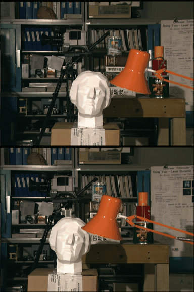
Image source: Middlebury Stereo Datasets (University of Tsukuba)
tsukuba_left = cv2.imread('../img/tsukuba_left.png', cv2.IMREAD_GRAYSCALE)
tsukuba_right = cv2.imread('../img/tsukuba_right.png', cv2.IMREAD_GRAYSCALE)

fig, axes = plt.subplots(1, 2, figsize=(7, 3.5))
axes[0].imshow(tsukuba_left, cmap='gray')
axes[0].set_title('Left photo', fontsize=9)
axes[1].imshow(tsukuba_right, cmap='gray')
axes[1].set_title('Right photo', fontsize=9)
for ax in axes:
    ax.axis('off')
plt.tight_layout()
plt.show()

num_disp = 64  # must be divisible by 16; large enough that the nearest surfaces don't clip the search range
stereo = cv2.StereoBM_create(numDisparities=num_disp, blockSize=15)
disp_lr = stereo.compute(tsukuba_left, tsukuba_right).astype(np.float32) / 16.0
disp_rl = stereo.compute(tsukuba_right[:, ::-1], tsukuba_left[:, ::-1]).astype(np.float32) / 16.0
disp_rl = disp_rl[:, ::-1]

stereo_checked = cv2.StereoBM_create(numDisparities=num_disp, blockSize=15)
stereo_checked.setDisp12MaxDiff(1)
disp_checked = stereo_checked.compute(tsukuba_left, tsukuba_right).astype(np.float32) / 16.0

changed = disp_lr != disp_checked
print(f'pixels changed by the consistency check: {changed.sum()} / {changed.size} ({100 * changed.sum() / changed.size:.1f}%)')

fig, axes = plt.subplots(1, 3, figsize=(10, 3.5))
for ax, d, title in zip(axes, [disp_lr, disp_rl, disp_checked],
                         ['Left-to-right disparity', 'Right-to-left disparity', 'After consistency check']):
    im = ax.imshow(np.where(d >= 0, d, np.nan), cmap=invalid_cmap, vmin=0, vmax=num_disp)
    ax.set_title(title, fontsize=9)
    ax.axis('off')
plt.colorbar(im, ax=axes, orientation='vertical', fraction=0.046, pad=0.04, label='disparity (px)')
plt.show()

The lamp, the nearest object in the scene, stands out with the largest disparity; the bookshelves recede smoothly behind it. Only about 1% of pixels get flagged, so the third panel looks almost the same as the first at a glance — but that speckle is concentrated exactly along depth discontinuities throughout the scene: book spines, shelf edges, the head's silhouette, wherever a window straddles two different depths or one camera sees something the other doesn't.
From disparity to depth map
Given a focal length and baseline (in whatever consistent units), $Z = fB/d$ converts a disparity map directly into a metric depth map.
focal_length_px = 500.0
baseline_m = 0.1

valid = disparity_bm > 0
depth_m = np.full_like(disparity_bm, np.nan)
depth_m[valid] = focal_length_px * baseline_m / disparity_bm[valid]

plt.imshow(depth_m, cmap='viridis_r')
plt.colorbar(label='estimated depth (m)')
plt.title('Depth map (nearer = brighter)')
plt.axis('off')
plt.show()

step = 3  # subsample for a readable, fast-to-render point cloud
ys, xs = np.mgrid[0:depth_m.shape[0]:step, 0:depth_m.shape[1]:step]
zs = depth_m[::step, ::step]
valid_pts = ~np.isnan(zs)

fig = plt.figure(figsize=(6, 5))
ax = fig.add_subplot(projection='3d')
sc = ax.scatter(xs[valid_pts], ys[valid_pts], zs[valid_pts], c=zs[valid_pts], cmap='viridis_r', s=3)
ax.set_xlabel('x (px)')
ax.set_ylabel('y (px)')
ax.set_zlabel('depth (m)')
ax.invert_yaxis()  # match image row convention (row 0 at top)
ax.invert_zaxis()  # nearer (smaller depth) points appear higher, like the disparity peaks above
ax.view_init(elev=20, azim=-60)
#fig.colorbar(sc, ax=ax, shrink=0.6, label='depth (m)')
ax.set_title('The depth map, lifted into 3D')
plt.tight_layout()
plt.show()

The same numbers, viewed as points floating in space instead of colors on a flat image, make the "planes" in this synthetic scene literal: three flat terraces at three different heights, with the holes where StereoBM had no confident match cut cleanly out of each one.
Exercise
- Replace the random-texture
leftimage with a flat gray region for the background (keeping the two rectangles textured). Runcv2.StereoBMagain and describe what happens to the disparity estimate over the flat area — this is the aperture problem from Lesson 20, now in a stereo-matching context. - Try
cv2.StereoSGBM_create(semi-global block matching, which enforces smoothness across neighboring disparities rather than matching each pixel completely independently) in place ofStereoBM. Compare the amount of speckle noise in flat/background regions between the two methods. - Increase
baseline_min the depth conversion. How does the estimated depth map change, and why would a wider-baseline stereo rig give more precise depth estimates for distant objects (at the cost of a larger minimum-distance blind spot, due to disparity ranges and occlusion, near the cameras)?