

Lesson 46: The Transformer Architecture
Lesson 45 introduced the attention operation. A Transformer (Vaswani et al., 2017★) wraps that operation into a reusable block and stacks many of them. This lesson builds the Transformer encoder which includes: multi-head attention (so a layer can track several kinds of relationships at once), the encoder block that wires multi-head attention together with layer normalization and a per-position feedforward network using residual connections (Lesson 37); along with positional encoding (to fix the fact that attention otherwise treats a sequence as an unordered set).
import numpy as np
import torch
import torch.nn as nn
import torch.nn.functional as F
import matplotlib.pyplot as plt
Multi-head attention
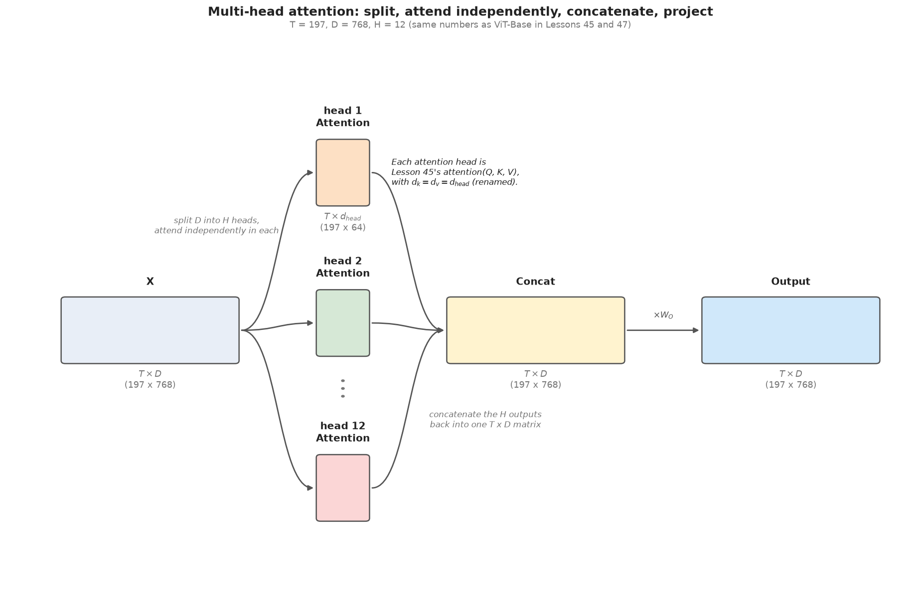
A single attention operation computes a similarity between every pair of positions. Multi-head attention splits the model dimension into several smaller chunks (heads), runs attention independently within each, and concatenates the results — letting different heads specialize in different kinds of relationships (e.g., one head might track nearby positions, another might track a specific long-range dependency) instead of averaging everything into one pattern.
The diagram below illustrates the idea, reusing the dimensions from Lesson 45 (sequence length T=197, number of features D=768) and sets the number of heads H=12, which is from ViT-Base's real head count (Lesson 47, coming up next). Each head is Lesson 45's attention(Q, K, V) pipeline, run once per head, with d_k = d_v = d_head (renamed, since every head here shares their width). After concatenating the H heads back into a T×D matrix, an additional learned linear layer — the output projection $W_O$, a D×D matrix — mixes information across heads before the result leaves the block. In the diagram below, each box indicates a tensor, and the arrows show the computation connecting them.
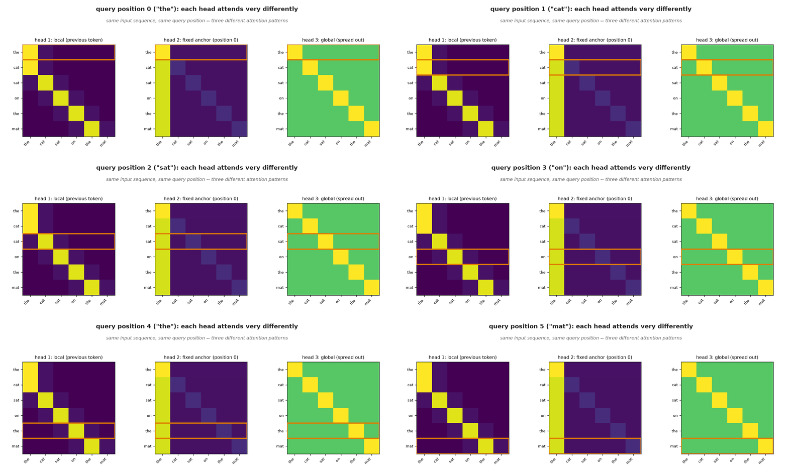
Why bother with multiple heads instead of one larger attention operation? Because each head is free to learn a completely different attention pattern from the same input. The animation below shows three illustrative heads (hand-constructed here, not trained, purely to make the point visible) attending very differently to the same query position — one local, one fixed on a single anchor token, one spread broadly across the sequence:
The cell below implements multi-head attention from scratch and validates it against PyTorch's own nn.MultiheadAttention.
D, H = 768, 12  # same ViT-Base numbers as the diagram above

def multihead_attention(x, mha):
    B, T, _ = x.shape  # batch dimension, and sequence length
    d_head = D // H  # head dimension is the feature dimension divided by the number of heads
    Wq, Wk, Wv = mha.in_proj_weight.chunk(3, dim=0)
    bq, bk, bv = mha.in_proj_bias.chunk(3, dim=0)
    Q = (x @ Wq.T + bq).view(B, T, H, d_head).transpose(1, 2)
    K = (x @ Wk.T + bk).view(B, T, H, d_head).transpose(1, 2)
    V = (x @ Wv.T + bv).view(B, T, H, d_head).transpose(1, 2)
    scores = Q @ K.transpose(-2, -1) / np.sqrt(d_head)
    weights = F.softmax(scores, dim=-1)
    out = (weights @ V).transpose(1, 2).reshape(B, T, D)
    return out @ mha.out_proj.weight.T + mha.out_proj.bias  # output projection

mha_torch = nn.MultiheadAttention(D, H, batch_first=True)

torch.manual_seed(0)
x = torch.randn(2, 5, D)
out_manual = multihead_attention(x, mha_torch)
out_torch, _ = mha_torch(x, x, x, need_weights=False)

print(f'model dim = {D}, heads = {H}, dim per head = {D // H}')
print(f'max abs diff vs nn.MultiheadAttention: {(out_manual - out_torch).abs().max().item():.2e}')
The encoder block
A single Transformer layer wires multi-head attention (just covered) together with a small per-position feedforward network, using two residual connections (Lesson 37), each followed by a normalization step:
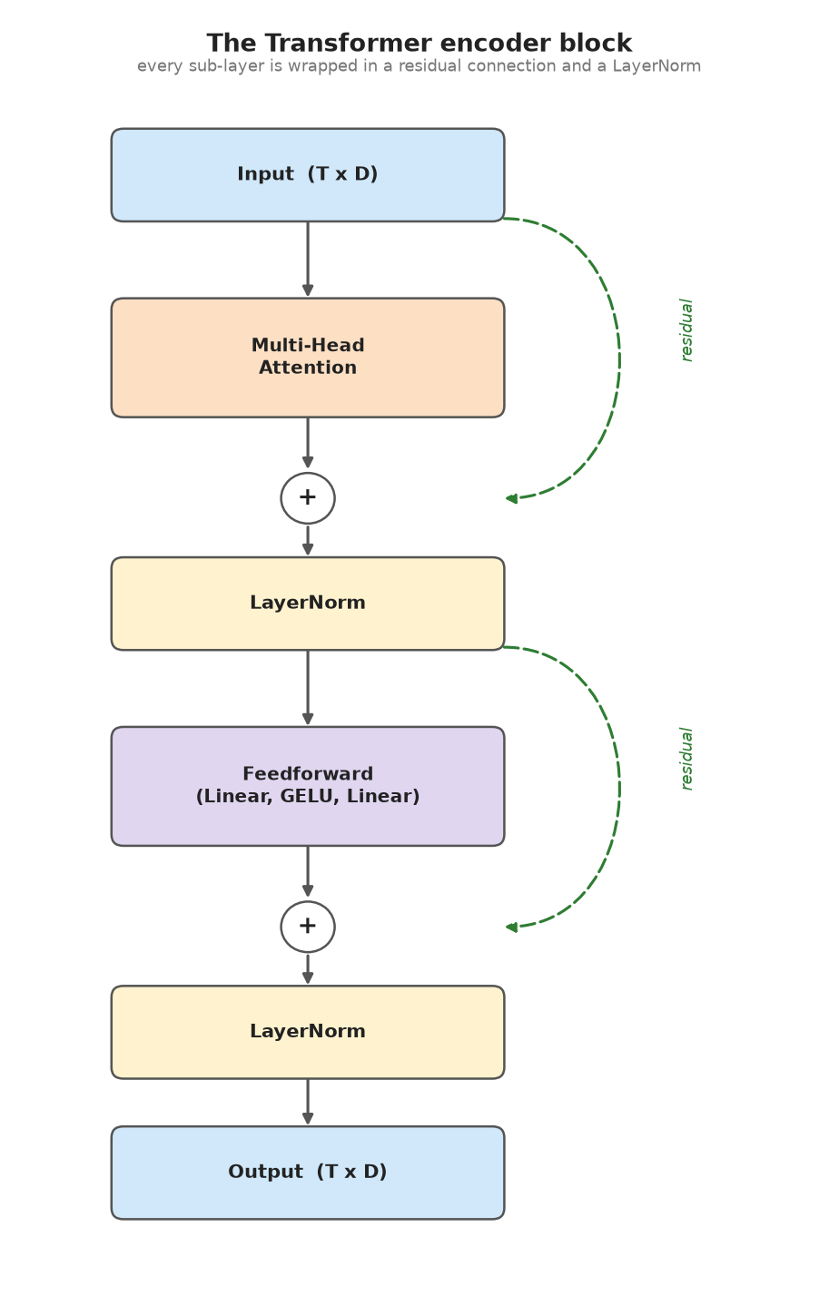
Two pieces of the diagram haven't been explained yet: layer normalization, and the feedforward network. The next two sections cover each of those in turn, then assemble the whole block in code.
Layer normalization
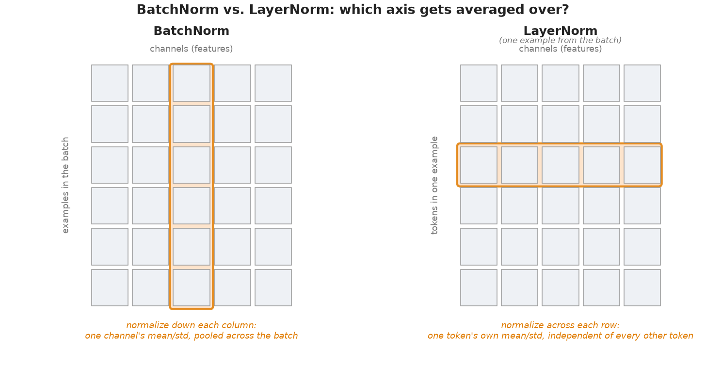
Lesson 37 covered the two-step recipe of batch normalization: first normalize, then apply a learned scale and shift. In the encoder block above, each "add & norm" wraps its sub-layer in layer normalization (Ba, Kiros & Hinton, 2016★, "LayerNorm"). LayerNorm is almost exactly the same as BatchNorm — the only thing that changes is which axis gets averaged over. BatchNorm pools a channel's mean/std across every example in the batch (different, unrelated images); whereas LayerNorm pools a token's mean/std across its own D feature channels — different positions within the same single example, never looking at any other example in the batch at all:
For a token with feature vector $x \in \mathbb{R}^D$:
$$\mu = \frac{1}{D}\sum_{d=1}^{D} x_d, \qquad \sigma^2 = \frac{1}{D}\sum_{d=1}^{D} (x_d - \mu)^2, \qquad \text{LayerNorm}(x) = \gamma \odot \frac{x - \mu}{\sqrt{\sigma^2 + \epsilon}} + \beta$$
where $\gamma, \beta \in \mathbb{R}^D$ are learned (shared across every token and every position), exactly as BatchNorm's $\gamma, \beta$ are learned per channel.
Why LayerNorm, not BatchNorm, for a Transformer encoder? BatchNorm's statistics depend on which other examples happen to be in the current batch, so it behaves differently at train time (use the current batch's mean/std) than at test time (fall back to a running average accumulated during training) — exactly the model.eval() distinction from Lesson 35. Forget to switch modes and BatchNorm silently misbehaves. LayerNorm avoids this problem: since it only looks at a token's own D channels, that computation is available in full for every single token (train or test) no matter the batch size or which other examples are present — so there's no batch-dependent statistic to estimate, no running average to maintain, and no train/eval distinction at all. The same formula runs in both modes.
x_ln = torch.randn(3, 5, D)  # (batch, T, D) -- same convention as the rest of this lesson

ln = nn.LayerNorm(D)
out_torch = ln(x_ln)

# from scratch: normalize each token over its own D feature channels (the last axis)
mean = x_ln.mean(dim=-1, keepdim=True)
var = x_ln.var(dim=-1, unbiased=False, keepdim=True)
x_norm = (x_ln - mean) / torch.sqrt(var + ln.eps)
out_manual = ln.weight * x_norm + ln.bias

print(f'max abs diff vs nn.LayerNorm: {(out_manual - out_torch).abs().max().item():.2e}')
print(f'per-token mean before (sample 0): {x_ln[0].mean(dim=-1).detach().numpy().round(3)}')
print(f'per-token std before (sample 0):  {x_ln[0].std(dim=-1, unbiased=False).detach().numpy().round(3)}')
print(f'per-token mean after (sample 0):  {out_torch[0].mean(dim=-1).detach().numpy().round(3)}')
print(f'per-token std after (sample 0):   {out_torch[0].std(dim=-1, unbiased=False).detach().numpy().round(3)}')
The feedforward network
Each encoder block also applies a small position-wise feedforward network after attention, which is two linear layers with a nonlinearity in between:
$$\text{FFN}(x) = \text{Linear}_2\big(\text{activation}(\text{Linear}_1(x))\big)$$
The first layer expands the hidden dimension D to rD, where r=4 is an expansion factor; the second layer then projects the activated result back down to D so the block's output shape matches its input. These two linear layers with a nonlinearity between them, mixing channels, is reminiscent of Lesson 37's squeeze-and-excitation (SE) block (Hu, Shen & Sun, 2018★). The SE block shrinks first (C → C/r) then expands (C/r → C) — a bottleneck designed to compactly summarize the information so that the network doesn't memorize an overly complex representation. (Since SE operates on a CNN feature map, C is the channel count, analogous to our feature dimension D here.) The FFN does the opposite, growing first (D → rD) then shrinking (rD → D) — to let an entirely new representation be computed at every position. That's the same intuition as Lesson 32's MLP: a wider hidden layer gives the nonlinearity more room to bend and fold the representation space before projecting back down.
Applied position-wise. This network runs independently at every position, using the same weights everywhere, with zero mixing across positions — attention is the only place information moves between positions anywhere in the block. That makes it mathematically identical to a 1x1 convolution across the sequence: a 1x1 conv's output at each location only looks at that location's own channels, with weights shared across every location, exactly like Linear applied position-wise.
The code below verifies that a position-wise Linear is identical to a 1x1 convolution.
DD = 4 * D  # ViT-Base's real feedforward width, introduced above

ffn_linear = nn.Sequential(nn.Linear(D, DD), nn.GELU(), nn.Linear(DD, D))
ffn_conv = nn.Sequential(nn.Conv1d(D, DD, kernel_size=1), nn.GELU(), nn.Conv1d(DD, D, kernel_size=1))

# copy weights across: Conv1d's (out, in, 1) is just Linear's (out, in) with a trailing axis
with torch.no_grad():
    ffn_conv[0].weight.copy_(ffn_linear[0].weight.unsqueeze(-1))
    ffn_conv[0].bias.copy_(ffn_linear[0].bias)
    ffn_conv[2].weight.copy_(ffn_linear[2].weight.unsqueeze(-1))
    ffn_conv[2].bias.copy_(ffn_linear[2].bias)

x3 = torch.randn(2, 6, D)
out_linear = ffn_linear(x3)
out_conv = ffn_conv(x3.transpose(1, 2)).transpose(1, 2)  # Conv1d expects (B, channels, T)

print(f'max abs diff (Linear-based FFN vs 1x1-Conv-based FFN): {(out_linear - out_conv).abs().max().item():.2e}')
The nonlinearity. Transformers replace Lesson 32's ReLU with Gaussian Error Linear Unit (GELU) (Hendrycks & Gimpel, 2016★). GELU is a smoother version of ReLU: instead of a hard cutoff at zero, it weights its input by how likely a standard normal variable is to fall below it:
$$\text{GELU}(u) = u \cdot \Phi(u), \qquad \Phi(u) = P(Z \le u) \text{ for } Z \sim \mathcal{N}(0, 1)$$
Note: In more recent transformers, SwiGLU has replaced GELU — a detail beyond this lesson.
def gelu_manual(u):
    phi = 0.5 * (1 + torch.erf(u / np.sqrt(2)))
    return u * phi

gelu_torch = nn.GELU()

u = torch.linspace(-4, 4, 200)
out_manual = gelu_manual(u)
out_torch = gelu_torch(u)
print(f'max abs diff vs nn.GELU: {(out_manual - out_torch).abs().max().item():.2e}')

plt.figure(figsize=(5, 3.5))
plt.plot(u, torch.relu(u), label='ReLU', linestyle='--')
plt.plot(u, out_torch, label='GELU')
plt.axhline(0, color='gray', linewidth=0.8)
plt.xlabel('u'); plt.ylabel('activation(u)')
plt.legend()
plt.title('GELU vs. ReLU')
plt.show()

Assembling the encoder block
With multi-head attention, layer normalization, the feedforward network, and GELU all covered, here's the block from the diagram above, implemented and validated against PyTorch's own nn.TransformerEncoderLayer:
class EncoderBlock(nn.Module):
    def __init__(self, D, H, FF):
        super().__init__()
        self.mha = nn.MultiheadAttention(D, H, batch_first=True)
        self.ln1 = nn.LayerNorm(D)
        self.ff = nn.Sequential(nn.Linear(D, FF), nn.GELU(), nn.Linear(FF, D))
        self.ln2 = nn.LayerNorm(D)

    def forward(self, x):
        attn_out, _ = self.mha(x, x, x, need_weights=False)
        x = self.ln1(x + attn_out)   # residual + norm around attention
        ff_out = self.ff(x)
        x = self.ln2(x + ff_out)     # residual + norm around the feedforward network
        return x

block = EncoderBlock(D, H, DD)
layer_torch = nn.TransformerEncoderLayer(d_model=D, nhead=H, dim_feedforward=DD,
                                          batch_first=True, dropout=0.0, activation='gelu')
layer_torch.eval()

# copy torch's weights into our block so the two are directly comparable
block.mha.load_state_dict(layer_torch.self_attn.state_dict())
block.ln1.load_state_dict(layer_torch.norm1.state_dict())
block.ln2.load_state_dict(layer_torch.norm2.state_dict())
block.ff[0].load_state_dict({'weight': layer_torch.linear1.weight, 'bias': layer_torch.linear1.bias})
block.ff[2].load_state_dict({'weight': layer_torch.linear2.weight, 'bias': layer_torch.linear2.bias})

x2 = torch.randn(2, 6, D)
out_block = block(x2)
out_layer = layer_torch(x2)
print(f'encoder block max abs diff vs nn.TransformerEncoderLayer: {(out_block - out_layer).abs().max().item():.2e}')
print(f'output shape unchanged from input: {tuple(out_block.shape)} == {tuple(x2.shape)}')
The block's output has exactly the same shape as its input — same trick as Lesson 37's residual block, and for the same reason: it means blocks can be stacked arbitrarily deep, each one refining the same sequence of tokens, without any reshaping between them. A full Transformer encoder is just N copies of this block stacked in sequence (nn.TransformerEncoder in PyTorch). Vision Transformers (Lesson 47) reuse this block almost unchanged — the only real difference is what gets fed in as the initial sequence of tokens.
Positional encoding
Attention computes similarity between content vectors — nothing about the formula from Lesson 45 refers to where in the sequence a position sits. Permute the input sequence, and attention's output permutes along with it, identically: it is fundamentally a set operation, blind to order. Positional encoding fixes this by adding a unique, deterministic pattern to each position before attention runs, so position becomes part of what gets compared. The original Transformer's choice is a fixed (not learned) sinusoid at multiple frequencies:
$$PE_{(pos, 2i)} = \sin(pos / 10000^{2i/D}), \qquad PE_{(pos, 2i+1)} = \cos(pos / 10000^{2i/D})$$
def positional_encoding(T, D):
    pos = torch.arange(T).unsqueeze(1).float()
    i = torch.arange(D).unsqueeze(0).float()
    angle_rates = 1.0 / (10000 ** (2 * (i // 2) / D))
    angles = pos * angle_rates
    pe = torch.zeros(T, D)
    pe[:, 0::2] = torch.sin(angles[:, 0::2])
    pe[:, 1::2] = torch.cos(angles[:, 1::2])
    return pe

pe = positional_encoding(50, 32)
plt.figure(figsize=(6, 4))
plt.imshow(pe.numpy().T, cmap='RdBu', aspect='auto')
plt.xlabel('position'); plt.ylabel('encoding dimension')
plt.title('Sinusoidal positional encoding')
plt.colorbar(fraction=0.046)
plt.show()

Does this actually matter? A task that requires knowing order
Build a task that's impossible to solve from content alone: a fixed vector A and a fixed vector B appear at two random positions in a noisy sequence, and the label is simply "does A appear before B?" A model that mean-pools attention output over the sequence can only tell which two tokens are present, never their order, unless position is somehow injected.
T, D = 8, 32  # smaller than the D=768 used above -- this cell trains 10 models from scratch, so speed matters
vec_a, vec_b = torch.randn(D), torch.randn(D)

def make_order_dataset(rng, n):
    X, y = [], []
    for _ in range(n):
        pos_a, pos_b = rng.choice(T, size=2, replace=False)
        seq = torch.randn(T, D) * 0.1
        seq[pos_a] = vec_a
        seq[pos_b] = vec_b
        X.append(seq)
        y.append(1.0 if pos_a < pos_b else 0.0)
    return torch.stack(X), torch.tensor(y, dtype=torch.float32)

rng = np.random.default_rng(3)
X_train, y_train = make_order_dataset(rng, 400)
X_test, y_test = make_order_dataset(rng, 150)

class TinyAttnClassifier(nn.Module):
    def __init__(self, use_pos_enc):
        super().__init__()
        self.use_pos_enc = use_pos_enc
        self.mha = nn.MultiheadAttention(D, 4, batch_first=True)
        self.fc = nn.Sequential(nn.Linear(D, 16), nn.ReLU(), nn.Linear(16, 1))
        if use_pos_enc:
            self.register_buffer('pe', positional_encoding(T, D))

    def forward(self, x):
        if self.use_pos_enc:
            x = x + self.pe
        attn_out, _ = self.mha(x, x, x, need_weights=False)
        return self.fc(attn_out.mean(dim=1)).squeeze(-1)

def train_eval(use_pos_enc, seed, epochs=300, lr=0.01):
    torch.manual_seed(seed)
    model = TinyAttnClassifier(use_pos_enc)
    opt = torch.optim.Adam(model.parameters(), lr=lr)
    for _ in range(epochs):
        opt.zero_grad()
        loss = F.binary_cross_entropy_with_logits(model(X_train), y_train)
        loss.backward()
        opt.step()
    with torch.no_grad():
        return ((model(X_test) > 0).float() == y_test).float().mean().item()

no_pe_accs = [train_eval(False, seed) for seed in range(5)]
pe_accs = [train_eval(True, seed) for seed in range(5)]

print(f'without positional encoding: mean test acc = {np.mean(no_pe_accs):.1%}  (+/- {np.std(no_pe_accs):.1%})')
print(f'with positional encoding:    mean test acc = {np.mean(pe_accs):.1%}  (+/- {np.std(pe_accs):.1%})')
Without positional encoding, the model is stuck at chance — it can only report which two tokens showed up, but not their relative order. Adding the fixed sinusoid gives every position a distinct signature the model can key off, and the task becomes trivial.
Recap, and what's next
Everything in this lesson has been about the Transformer encoder: a block that reads an entire sequence at once (bidirectional, no masking) and produces a representation of it — exactly what Lesson 47's Vision Transformer builds on directly. The literature also talks about Transformer decoders, and about encoder-decoder, encoder-only, and decoder-only architectures. The distinction matters a lot (it's how a Transformer actually generates text, an image caption, or anything else one step at a time), but it leans on a clean notion of "encoding" versus "decoding" that Lesson 48's autoencoders will give us first. Lesson 58 picks the thread back up once that vocabulary is in place, and Lesson 59 completes it.
Exercises
- Change
H(heads) from 12 to 1, keepingD=768fixed, and rerun the multi-head attention validation. With a single head, is there still a meaningful difference from Lesson 45's single-headattentionfunction? - In the order-detection task, change
T(sequence length) from 8 to 32. Does the with-positional-encoding model's accuracy hold up, or does the longer sequence make the task harder in a way positional encoding alone doesn't fix? EncoderBlockabove uses "post-norm" (LayerNormapplied after the residual add, matching the original 2017 paper). Many modern Transformers use "pre-norm" instead:x = x + self.mha(self.ln1(x)). Implement pre-norm and compare the two at greater depth (stack 10 blocks) — does one train more stably, echoing Lesson 37's vanishing-gradient story?