

Lesson 47: Vision Transformers (ViT)
Lesson 46's Transformer encoder operates on a sequence of vectors (called tokens). Transformers were originally designed to process language, where the tokens correspond roughly to syllables or words. Since an image is inherently 2D rather than a 1D sequence, the Vision Transformer (Dosovitskiy et al., 2020★) turns it into one: chop the image into fixed-size patches, flatten and linearly embed each patch into a vector (or token), and feed the resulting sequence into an ordinary Transformer encoder, exactly as built in Lesson 46. This lesson builds that pipeline, and then runs the exact translation-generalization test from Lesson 34 to show precisely what a Transformer gives up by dropping convolution's built-in inductive bias.
import numpy as np
import torch
import torch.nn as nn
import torch.nn.functional as F
import matplotlib.pyplot as plt
Patchify: turning an image into a sequence
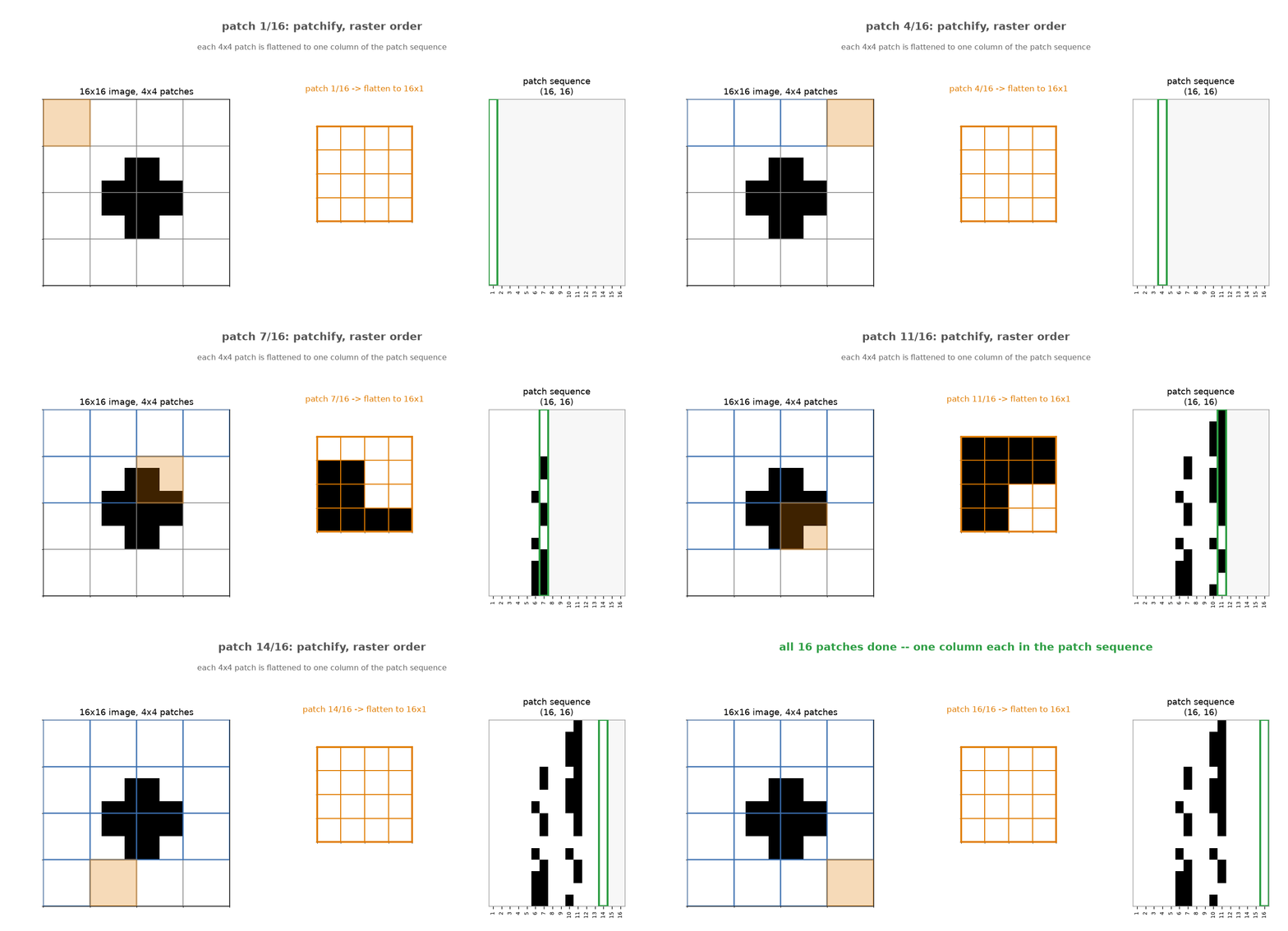
Split a 16x16 image into 4x4 patches and flatten each one into a 16-element vector, yielding a sequence of 16 patches — patchify is a pure reshape: no weights, no computation.
def patchify(img, patch_size):
    B, C, H, W = img.shape
    P = patch_size
    patches = img.unfold(2, P, P).unfold(3, P, P)  # (B, C, H/P, W/P, P, P)
    patches = patches.contiguous().view(B, C, -1, P, P).permute(0, 2, 1, 3, 4)
    return patches.reshape(B, -1, C * P * P)  # (B, num_patches, C*P*P)

img = torch.randn(2, 1, 16, 16)
patches = patchify(img, patch_size=4)
print(f'image {tuple(img.shape)} -> patch sequence {tuple(patches.shape)}  '
      f'({(16 // 4) ** 2} patches of {1 * 4 * 4} values each)')
The animation below carves a 16x16 image into its 16 patches one at a time, flattening each into a column of the growing patch sequence.
Linear embedding: turning patches into tokens
Each flattened patch is still just raw pixel values, not yet a token in the Transformer sense. The embedding step maps every patch through a shared linear layer, nn.Linear(16, 32), turning patchify's (16, 16) patch sequence into an embedded (32, 16) sequence of tokens. (Each of the 16 tokens is a 32-element vector.)
Stack all 16 patches as columns of a (16, 16) matrix P, then embed every patch is a single matrix multiply:
$$X_{\text{embed}} = W P, \qquad W \in \mathbb{R}^{32 \times 16}, \quad P \in \mathbb{R}^{16 \times 16}, \quad X_{\text{embed}} \in \mathbb{R}^{32 \times 16}$$
where W is the nn.Linear's (32, 16) weight matrix — the same W is applied to every column of P. That's what "shared weights" means here: one matrix, reused identically across all 16 patches, the same idea as a conv kernel reused at every spatial location. In fact this computation is exactly equivalent to a strided convolution with a kernel the same size as the stride (nn.Conv2d(..., kernel_size=P, stride=P)) — both slide a non-overlapping window and apply the same weights at every position.
patch_dim, embed_dim = 16, 8
linear_embed = nn.Linear(patch_dim, embed_dim)
conv_embed = nn.Conv2d(1, embed_dim, kernel_size=4, stride=4)
with torch.no_grad():
    conv_embed.weight.copy_(linear_embed.weight.view(embed_dim, 1, 4, 4))
    conv_embed.bias.copy_(linear_embed.bias)

out_linear = linear_embed(patches)
out_conv = conv_embed(img).flatten(2).transpose(1, 2)
print(f'linear-on-patches vs. strided-conv max abs diff: {(out_linear - out_conv).abs().max().item():.2e}')
The [CLS] token, and assembling a full ViT
To turn a sequence of patch embeddings (tokens) into a single whole-image prediction, ViT prepends one extra, learned "classification" token to the sequence before running the Transformer encoder (Lesson 46). After attention has let it gather information from every patch, that one token's final output is what the classification head reads. But first, positional encoding (Lesson 46) is added so patch order (i.e. patch location) isn't invisible to attention.
The class below, ToyViT, assembles exactly that: a linear patch embedding, a prepended [CLS] token, positional encoding, and a stack of ordinary Transformer encoder layers reading off that one token's final output. Every animation in this lesson traces this exact model's forward pass.
def positional_encoding(T, D):
    pos = torch.arange(T).unsqueeze(1).float()
    i = torch.arange(D).unsqueeze(0).float()
    angle_rates = 1.0 / (10000 ** (2 * (i // 2) / D))
    angles = pos * angle_rates
    pe = torch.zeros(T, D)
    pe[:, 0::2] = torch.sin(angles[:, 0::2])
    pe[:, 1::2] = torch.cos(angles[:, 1::2])
    return pe

class ToyViT(nn.Module):
    def __init__(self, img_size=16, patch_size=4, in_ch=1, embed_dim=32, n_heads=4, n_layers=2):
        super().__init__()
        self.patch_size = patch_size
        n_patches = (img_size // patch_size) ** 2
        patch_dim = in_ch * patch_size * patch_size
        self.embed = nn.Linear(patch_dim, embed_dim)
        self.cls_token = nn.Parameter(torch.randn(1, 1, embed_dim) * 0.02)
        self.register_buffer('pos_enc', positional_encoding(n_patches + 1, embed_dim))
        layer = nn.TransformerEncoderLayer(embed_dim, n_heads, dim_feedforward=embed_dim * 2,
                                            batch_first=True, dropout=0.0)
        self.encoder = nn.TransformerEncoder(layer, num_layers=n_layers)
        self.head = nn.Linear(embed_dim, 2)

    def forward(self, x):
        p = patchify(x, self.patch_size)
        tok = self.embed(p)
        cls = self.cls_token.expand(x.shape[0], -1, -1)
        tok = torch.cat([cls, tok], dim=1) + self.pos_enc
        out = self.encoder(tok)
        return self.head(out[:, 0])  # classify from the [CLS] token's output

model = ToyViT()
x = torch.randn(3, 1, 16, 16)
out = model(x)
print(f'ToyViT: input {tuple(x.shape)} -> output {tuple(out.shape)}  (two logits per image, one per class)')
The Transformer encoder
ToyViT.encoder is nothing new: it's exactly the nn.TransformerEncoder built in Lesson 46, stacked n_layers=2 deep, running on the (32, 17) sequence X assembled above. Self-attention, add-&-norm, feed-forward, and add-&-norm are all shape-preserving, so X stays exactly (32, 17) through both layers — only the content changes, as every token's representation is updated by attending to every other token (including [CLS], which is what lets it gather information from the whole image).
Extraction and classification
ToyViT.head reads out[:, 0] — the [CLS] column — and maps it with nn.Linear(32, 2) down to (2,): two logits, one per class, normalized by softmax into a probability distribution over the two classes {plus, circle}. All other columns — the 16 patch tokens' final states — are simply discarded.
That has a direct consequence for training: since self-attention, add-&-norm, and feed-forward are all shape-preserving, the encoder's output still has 17 columns, so what happens to the other 16? Nothing the loss cares about, directly: F.cross_entropy is computed from head(out[:, 0]) alone, so autograd only routes a gradient into that one column of the encoder's final output — the other 16 columns' final-layer values get no gradient from this loss. Earlier-layer versions of those patch tokens still matter, since they were used as keys and values that [CLS] attended to — but their own final output is simply never graded against anything. That's precisely the gap that Lesson 49 (reconstruction) and Lesson 51 (self-distillation) each close in their own way, by building losses that do directly supervise the patch tokens.
Putting it all together: the full pipeline
The diagram below lays out that entire pipeline at a glance, one box per stage with every shape labeled — a static complement to the step-by-step animation further down.
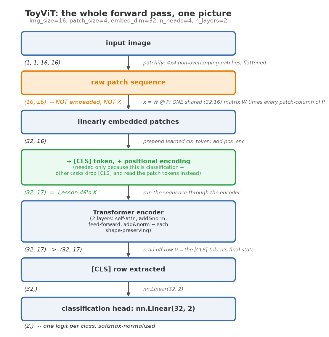
The animation below traces an example image through this exact ToyViT.forward call — inference only, ending on the classification head's output.

What convolution's inductive bias buys you
Lesson 34 trained a CNN and a flatten-based MLP on plus-vs-circle shapes at one range of positions, then tested both at unseen positions — the CNN generalized (global max pooling makes it exactly translation-invariant); the flatten-based MLP didn't (its first layer's weights are tied to absolute pixel coordinates). Rerun that exact experiment, swapping in ToyViT for the MLP.
A ViT has no built-in translation invariance either — patch embedding and positional encoding are both position-specific, same as the MLP's flattened input. The chief practical mechanism ViTs use to compensate is scale: pretraining on enormous datasets lets attention learn something like translation invariance from data, rather than getting it for free from the architecture the way a CNN does. On the tiny dataset in this course, expect that learning to fail.
def make_image(shape_type, cx, cy, size=16):
    img = np.zeros((size, size), dtype=np.float32)
    if shape_type == 'plus':
        img[cy-1:cy+2, cx-3:cx+4] = 1.0
        img[cy-3:cy+4, cx-1:cx+2] = 1.0
    else:
        yy, xx = np.mgrid[0:size, 0:size]
        img[((xx-cx)**2 + (yy-cy)**2) <= 9] = 1.0
    return img

def make_dataset(rng_local, n, position_range):
    imgs, labels = [], []
    for _ in range(n):
        shape_type = rng_local.choice(['plus', 'circle'])
        cx, cy = rng_local.integers(*position_range), rng_local.integers(*position_range)
        imgs.append(make_image(shape_type, cx, cy))
        labels.append(0 if shape_type == 'plus' else 1)
    return np.array(imgs, dtype=np.float32), np.array(labels, dtype=np.int64)

data_rng = np.random.default_rng(1)
X_train, y_train = make_dataset(data_rng, 300, (5, 11))   # training positions
X_test, y_test = make_dataset(data_rng, 150, (3, 5))       # UNSEEN positions

class CNNClassifier(nn.Module):
    def __init__(self):
        super().__init__()
        self.conv = nn.Sequential(
            nn.Conv2d(1, 8, 5, padding=2), nn.ReLU(), nn.MaxPool2d(2),
            nn.Conv2d(8, 16, 5, padding=2), nn.ReLU(), nn.AdaptiveMaxPool2d(1))
        self.fc = nn.Linear(16, 2)

    def forward(self, x):
        return self.fc(self.conv(x).flatten(1))

def train_and_eval(model_cls, Xtr, ytr, Xte, yte, seed, epochs=200, lr=0.001):
    torch.manual_seed(seed)
    model = model_cls()
    opt = torch.optim.Adam(model.parameters(), lr=lr)
    for _ in range(epochs):
        opt.zero_grad()
        loss = F.cross_entropy(model(Xtr), ytr)
        loss.backward()
        opt.step()
    with torch.no_grad():
        train_acc = (model(Xtr).argmax(1) == ytr).float().mean().item()
        test_acc = (model(Xte).argmax(1) == yte).float().mean().item()
    return train_acc, test_acc

Xtr_t = torch.tensor(X_train).unsqueeze(1); ytr_t = torch.tensor(y_train)
Xte_t = torch.tensor(X_test).unsqueeze(1); yte_t = torch.tensor(y_test)

for seed in range(3):
    vit_train, vit_test = train_and_eval(ToyViT, Xtr_t, ytr_t, Xte_t, yte_t, seed=seed)
    cnn_train, cnn_test = train_and_eval(CNNClassifier, Xtr_t, ytr_t, Xte_t, yte_t, seed=seed)
    print(f'seed={seed}: ViT train={vit_train:.1%} test(unseen positions)={vit_test:.1%}   '
          f'|   CNN train={cnn_train:.1%} test(unseen positions)={cnn_test:.1%}')
Both models fit the training positions perfectly, but the ViT collapses to chance-level (or worse) on unseen positions every time, while the CNN generalizes perfectly — reproducing Lesson 34's MLP-vs-CNN gap almost exactly, with the ViT standing in for the MLP. This is the well-documented empirical finding behind real ViTs: they need either far more training data, or heavy data augmentation, or a hybrid architecture that reintroduces some convolutional structure, to match a CNN's data efficiency on small-to-medium datasets — because a CNN's translation invariance is a hard architectural guarantee, while a ViT's has to be learned from examples. Only at the scale of hundreds of millions of images, ViTs match or beat CNNs.
Exercises
- Increase the training set size in
make_dataset(data_rng, 300, ...)from 300 to 3000 images at the same training positions. Does the ViT's unseen-position accuracy improve substantially, partially, or not at all — and what does that suggest about how much more data a ViT needs to compensate for its missing inductive bias? - Reduce
patch_sizefrom 4 to 2 (finer patches, longer sequence). Does finer patching help the ViT generalize better to unseen positions, or is the failure mode unrelated to patch resolution? - A "hybrid" architecture feeds a small CNN's feature map (instead of raw pixel patches) into a Transformer encoder, gaining some of the CNN's spatial inductive bias back. Sketch how you'd modify
ToyViT.forwardto patchify the output of a smallnn.Conv2dstack instead of the raw image.